2.3 Pandas - Machine Learning in the Geosciences

This section aims to provide new skills in python to handle structured, tabular data.

Learning outcome:

Manipulation of data frames (describing, filtering, ...)
Learn about Lambda functions
Intro to datetime objects
Plotting data from data frames (histograms and maps)
Introduction to Plotly
Introduction to CSV & Parquet

This tutorial can be offered in a 2-hour course. Sections are labeled as Level 1, 2, 3 in Section 1, 2, 3, and instructors may choose to leave higher levels for asynchronous, self-guided learning.

We will work on several structured data sets: sensor metadata, seismic data product (earthquake catalog).

First, we import all the modules we need:

🖥️ Lecture slides — Session 05 (Fri Oct 9)

import io
import os

import matplotlib.pyplot as plt
import numpy as np
import pandas as pd
import pooch
import requests

os.makedirs('data', exist_ok=True)

This notebook uses plotly to make interactive plots

import plotly.express as px
import plotly.io as pio
# pio.renderers.default = 'vscode' # writes as standalone html, 
# pio.renderers.default = 'iframe' # writes files as standalone html, 
# pio.renderers.default = 'png' # writes files as standalone png, 
# try notebook, jupyterlab, png, vscode, iframe

1 Pandas Fundamentals¶

1.1 Basics¶

The core pandas objects are Series and DataFrame. A Series is a one-dimensional labeled array. The DataFrame is a two-dimensional table whose columns are Series.

We can create a DataFrame composed of series from scratch using Python dictionary:

data = {
    'temperature' : [36,37,30,50],
    'precipitation':[3,1,0,0]
}
my_pd = pd.DataFrame(data)
print(my_pd)

   temperature  precipitation
0           36              3
1           37              1
2           30              0
3           50              0

Each (key,value) item in the dataframe corresponds to a value in data. To get the keys of the dataframe, type:

my_pd.keys()

Index(['temperature', 'precipitation'], dtype='str')

get a specific Series (different from the array)

print(my_pd.temperature[:])
print(type(my_pd.temperature[:]))

0    36
1    37
2    30
3    50
Name: temperature, dtype: int64
<class 'pandas.Series'>

to get the value of a specific key (e.g., temperature), at a specific index (e.g., 2) type:

print(my_pd.temperature[2])
print(type(my_pd.temperature[2]))

30
<class 'numpy.int64'>

1.2 Reading a DataFrame from a CSV file¶

We can read a pandas directly from a standard file. We will download a catalog of earthquakes with pooch, which caches the file in the local data/ folder.

ff = pooch.retrieve(
    url="https://raw.githubusercontent.com/UW-MLGEO/MLGeo-dataset/refs/heads/main/data/Global_Quakes_IRIS.csv",
    known_hash=None,
    fname="Global_Quakes_IRIS.csv",
    path="./data",
)
quake = pd.read_csv(ff)

Downloading data from 'https://raw.githubusercontent.com/UW-MLGEO/MLGeo-dataset/refs/heads/main/data/Global_Quakes_IRIS.csv' to file '/home/runner/work/mlgeo-book/mlgeo-book/book/Chapter2-DataManipulation/data/Global_Quakes_IRIS.csv'.

SHA256 hash of downloaded file: 4cd4369cf0b130420c830565a7e600fdf7c2f6e5317656e713b83f7c66849bf0
Use this value as the 'known_hash' argument of 'pooch.retrieve' to ensure that the file hasn't changed if it is downloaded again in the future.

Now you use the head function to display what is in the file

# enter answer here
quake.head()

Display the depth using two ways to use the pandas object

print(quake.depth)
print(quake['depth'])

0        34400.0
1        30100.0
2        16900.0
3       109400.0
4        25700.0
          ...   
1780     10000.0
1781    105000.0
1782    608510.0
1783     10000.0
1784     35440.0
Name: depth, Length: 1785, dtype: float64
0        34400.0
1        30100.0
2        16900.0
3       109400.0
4        25700.0
          ...   
1780     10000.0
1781    105000.0
1782    608510.0
1783     10000.0
1784     35440.0
Name: depth, Length: 1785, dtype: float64

Calculate basic statistic of the data using the function describe.

quake.describe()

Calculate mean and median of specific Series, for example depth.

# answer it here
print(quake.depth.mean())
print(quake.depth.median())

82773.18767507003
24400.0

1.3 Manipulating Pandas with Python¶

Classic functions¶

We will now practice how to modify the content of the DataFrame using functions. We will take the example where we want to change the depth values from meters to kilometers. First we can define this operation as a function

# this function converts a value in meters to a value in kilometers
m2km = 1000 # this is defined as a global variable
def meters2kilometers(x):
    return x/m2km

# now test it using the first element of the quake DataFrame
meters2kilometers(quake.depth[0])

np.float64(34.4)

# this function converts a value in meters to a value in kilometers
def meters2kilometers2(x):
    m2km = 1000 # this is defined as a global variable
    return x/m2km

Let’s define another function that uses a local instead of global variable

# Apply the meters2kilometers2 function to the 'depth' column and add it as a new column 'depth_km' to the quake DataFrame
quake['depth_km'] = quake['depth'].apply(meters2kilometers2)

# Display the first few rows to verify the new column
quake.head()

Lambda functions¶

We now discuss the lambda functions.

Lambda functions are small, anonymous functions in Python.
They are used for quick, simple operations without needing to define a full function using def.
In geoscience, where we deal with large datasets (e.g., climate data, seismic measurements), lambda functions allow us to process data efficiently.
Lambda functions in Pandas allow you to quickly transform, filter, or process this data with minimal code.
Please read additional tutorials from RealPython.

lambda x: x * 1.2

<function __main__.<lambda>(x)>

This lambda function multiplies any input x by 1.2, which could be useful for tasks like converting units (e.g., from km to m).

Below is an example on how to use lambda in a pandas dataframe. Example 1: The lambda function lambda x: (x - 32) * 5 / 9 converts Fahrenheit to Celsius for each value in the Temperature_F column.

import pandas as pd

# Sample DataFrame
data = {'Temperature_F': [32, 50, 77, 100]}
df = pd.DataFrame(data)

# Convert Fahrenheit to Celsius
df['Temperature_C'] = df['Temperature_F'].apply(lambda x: (x - 32) * 5 / 9)

print(df)

   Temperature_F  Temperature_C
0             32       0.000000
1             50      10.000000
2             77      25.000000
3            100      37.777778

# Now the equivalent in lambda is:
lambda_meters2kilometers = lambda x:x/1000
# x is the variable

Now apply the function to the entire series

# apply it to the entire series
lambda_meters2kilometers(quake.depth)

0        34.40
1        30.10
2        16.90
3       109.40
4        25.70
         ...  
1780     10.00
1781    105.00
1782    608.51
1783     10.00
1784     35.44
Name: depth, Length: 1785, dtype: float64

Lambda functions can take several inputs

# you can add several variables into lambda functions
remove_anything = lambda x,y:x-y
remove_anything(3,2)

1

This did not affect the values of the DataFrame, check it:

quake.depth

0        34400.0
1        30100.0
2        16900.0
3       109400.0
4        25700.0
          ...   
1780     10000.0
1781    105000.0
1782    608510.0
1783     10000.0
1784     35440.0
Name: depth, Length: 1785, dtype: float64

Instead, you could overwrite quake.depth=X. Try two approaches but just do it once! You can use python functions map (a function to apply functions that is generic to Python) and apply (a function to apply functions that is specific to Pandas).

Try map to apply a lambda function that rescale depth from meters to kilometers.

#type answer below
quake.depth=quake.depth.map(lambda x:x/1000)

Discuss in class: What happened to the depth field?

What happened to the original data frame?

Try apply to apply a lambda function that rescale depth from meters to kilometers. Here we only display the result without assigning it, because the previous cell already converted the column to kilometers.

# or like this (display only, the column is already in km)
quake.depth.apply(lambda x:x/1000)

0       0.03440
1       0.03010
2       0.01690
3       0.10940
4       0.02570
         ...   
1780    0.01000
1781    0.10500
1782    0.60851
1783    0.01000
1784    0.03544
Name: depth, Length: 1785, dtype: float64

Plot a histogram of the depth distributions using matplotlib function hist.

# answer here
plt.hist(quake.depth,100)
plt.grid(True)
plt.xlabel('Quake depth (km)')
plt.show()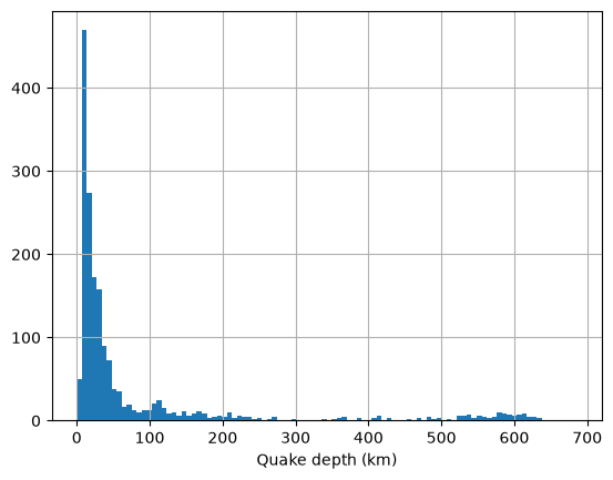

You can use the interactive plotting package Plotly. First we will show a histogram of the event depth using the function histogram.

fig = px.histogram(quake,   #specify what dataframe to use
             x="depth",  #specify the variable for the histogram 
             nbins=50,       #number of bins for the histogram 
             height=400,     #dimensions of the figure
             width=600);
fig.show()

Example 2: Conditional Logic for Earthquake Magnitude¶

You can use lambda functions to add conditional logic, such as classifying earthquake magnitudes into categories.

Scenario: You have a column Magnitude containing seismic event magnitudes, and you want to classify events as “Minor”, “Moderate”, or “Severe”.

# Classify earthquake magnitudes
quake['Category'] = quake['magnitude'].apply(lambda x: 'Minor' if x < 4.0 else ('Moderate' if x < 6.5 else 'Severe'))
quake.head()

We will now make a new plot of the location of the earthquakes. We will use Plotly tool.

The markersize will be scaled with the earthquake magnitude. To do so, we add a marker_size series in the DataFrame

quake['marker_size'] = quake['magnitude'].apply(lambda x: np.trunc(np.exp(x))) # add marker size as exp(mag)
quake['magnitude_bin'] = quake['magnitude'].apply(lambda x: 0.5*np.trunc(2*x)) # bin magnitude in 0.5 steps

# another way to do it
quake['marker_size'] = np.trunc(np.exp(quake['magnitude'])) # add marker size as exp(mag)
quake['magnitude_bin'] = 0.5*np.trunc(2*quake['magnitude']) # bin magnitude in 0.5 steps

1.4 Intermediate Manipulation with Pandas¶

You can also apply lambda functions to work with multiple columns, which is common in geoscientific datasets, where you might have spatial or temporal data.

Example 3: Calculating an Index Based on Multiple Measurements Scenario: You have rainfall (Rainfall_mm) and evaporation (Evaporation_mm) data, and you want to calculate the Net Water Balance for each record.

data = {'Rainfall_mm': [100, 80, 120], 'Evaporation_mm': [60, 70, 65]}
df = pd.DataFrame(data)

# Calculate Net Water Balance
df['Net_Water_Balance'] = df.apply(lambda row: row['Rainfall_mm'] - row['Evaporation_mm'], axis=1)

print(df)

   Rainfall_mm  Evaporation_mm  Net_Water_Balance
0          100              60                 40
1           80              70                 10
2          120              65                 55

In this example, lambda row: row['Rainfall_mm'] - row['Evaporation_mm'] calculates the net water balance by subtracting evaporation from rainfall for each record.

1.5 Advanced: Time Series Data Manipulation with Lambda Functions¶

Geoscientists frequently work with time series data (e.g., climate data). Lambda functions can be used for efficient data transformations within time series.

Example 4: Applying a Rolling Window Calculation Scenario: Suppose you have daily temperature data, and you want to calculate a 3-day rolling average.

# Sample daily temperature data
data = {'Date': pd.date_range(start='2023-09-01', periods=10, freq='D'),
        'Temperature_C': [20, 22, 23, 21, 19, 24, 25, 26, 22, 20]}
df = pd.DataFrame(data)

# Calculate 3-day rolling average using lambda
df['7_day_avg'] = df['Temperature_C'].rolling(window=3).apply(lambda x: x.mean())
df.head()

Here, lambda x: x.mean() calculates the rolling mean over a 3-day window for temperature data, which is essential in climate analysis for smoothing short-term fluctuations.

1.6 Aggregate function¶

The agg is a powerful method in Pandas that allows you to perform multiple operations on DataFrames and Series. You can apply one or more aggregation functions such as sum, mean, min, max, etc., on different columns or groups of data.

# Sample DataFrame
data = {
    'A': [1, 2, 3, 4],
    'B': [5, 6, 7, 8]
}
df = pd.DataFrame(data)

# Apply aggregation functions
result = df['A'].agg(['sum', 'mean'])
print(result)

sum     10.0
mean     2.5
Name: A, dtype: float64

Aggregating Multiple Columns with Multiple Functions¶

You can pass a dictionary to agg where the keys are column names and the values are the functions to be applied.

# Apply different functions to different columns
result = df.agg({'A': ['sum', 'mean'], 'B': ['min', 'max']})
print(result)

         A    B
sum   10.0  NaN
mean   2.5  NaN
min    NaN  5.0
max    NaN  8.0

In this example, column ‘A’ gets sum and mean, while column ‘B’ gets min and max.

You may also use custom functions

# Custom function to calculate range (max - min)
def data_range(x):
    return x.max() - x.min()

# Apply custom function
result = df.agg({'A': ['mean', data_range], 'B': data_range})
print(result)

              A    B
mean        2.5  NaN
data_range  3.0  3.0

2 Mapping using Plotly¶

Now we will plot the earthquakes locations on a map using the Plotly package. More tutorials on Plotly. The input of the function is self-explanatory and typical of Python’s function. The code documentation of Plotly scatter_geo lists the variables.

fig = px.scatter_geo(quake,
                     lat='latitude',lon='longitude', 
                     range_color=(6,9),
                     height=600, width=600,
                     size='marker_size', color='magnitude',
                     hover_name="description",
                     hover_data=['description','magnitude','depth']);
fig.update_geos(resolution=110, showcountries=True)
fig.update_geos(resolution=110, showcountries=True,projection_type="orthographic")
fig

The lambda function lambda x: 'Minor' if x < 4.0 else ('Moderate' if x < 6.5 else 'Severe') classifies earthquake magnitudes based on their values.

The data was sorted by time. We now want to sort and show the data instead by magnitude. We use the pandas function sort to create a new DataFrame with sorted values.

quakes2plot=quake.sort_values(by='magnitude_bin')
quakes2plot.head()

Now we will plot again using Plotly

fig = px.scatter_geo(quakes2plot,
                     lat='latitude',lon='longitude', 
                     range_color=(6,9),
                     height=600, width=600,
                     size='marker_size', color='magnitude',
                     hover_name="description",
                     hover_data=['description','magnitude','depth']);
fig.update_geos(resolution=110, showcountries=True)
# fig.update_geos(resolution=110, showcountries=True,projection_type="orthographic")

3 Create a Pandas from a generic text file.¶

The python package pandas is very useful to read csv files, but also many text files that are more or less formatted as one observation per row and one column for each feature.

As an example, we are going to look at the list of seismic stations from the Northern California seismic network, available here:

url = 'https://ncedc.org/ftp/pub/doc/NC.info/NC.channel.summary.day'

# this gets the file linked in the URL page and convert it to a string
s = requests.get(url).content

# this will convert the string, decode it , and make it a table
data = pd.read_csv(io.StringIO(s.decode('utf-8')), header=None, skiprows=2, sep=r'\s+', usecols=list(range(0, 13)))
# because columns/keys were not assigned, assign them now
data.columns = ['station', 'network', 'channel', 'location', 'rate', 'start_time', 'end_time', 'latitude', 'longitude', 'elevation', 'depth', 'dip', 'azimuth']

Let us look at the data. They are now stored into a pandas dataframe.

data.head()

We can output the first element of the DataFrame:

data.iloc[0]

station                       AAR
network                        NC
channel                       EHZ
location                       --
rate                          0.0
start_time    1976/07/20,17:38:00
end_time      1977/12/01,22:37:00
latitude                 39.27594
longitude              -121.02696
elevation                   911.0
depth                         0.0
dip                         -90.0
azimuth                       0.0
Name: 0, dtype: object

# display the type of each column
data.dtypes

station           str
network           str
channel           str
location          str
rate          float64
start_time        str
end_time          str
latitude      float64
longitude     float64
elevation     float64
depth         float64
dip           float64
azimuth       float64
dtype: object

data.iloc[:, 0]

0         AAR
1         AAR
2         AAR
3         AAR
4         AAR
         ... 
33375     WMP
33376     WMP
33377     WMP
33378     WSL
33379    WWVB
Name: station, Length: 33380, dtype: str

The start_time and end_time are stored as object (strings), so we cannot do datetime arithmetic on them yet. We convert them with pd.to_datetime and an explicit format string.

A caution about AI assistants: an AI assistant may fail at this conversion if you give it a vague prompt, for example by guessing the wrong format string or by silently dropping the out-of-range dates. Always check dtypes (and a few actual values) after any AI-written parsing code.

# convert start_time to datetime with an explicit format
data['start_time'] = pd.to_datetime(data['start_time'], format='%Y/%m/%d,%H:%M:%S')

The end times need one extra step. NCEDC marks channels that are still operating with the placeholder end date 3000/01/01. That is not a real end date. We pass errors='coerce' so any unparseable entry becomes NaT (not-a-time) instead of raising an error; on older pandas versions, which stored timestamps at nanosecond resolution, year 3000 was out of range and was coerced this way. Pandas 3 parses timestamps at microsecond resolution, so year 3000 now parses fine, and we set the placeholder to NaT explicitly. This is deliberate and meaningful: after the conversion, NaT in end_time identifies the channels that are still running.

data['end_time'] = pd.to_datetime(data['end_time'], format='%Y/%m/%d,%H:%M:%S', errors='coerce')
# the year-3000 placeholder is not a real end date: mark those channels as still operating
data.loc[data['end_time'] == pd.Timestamp('3000-01-01'), 'end_time'] = pd.NaT

data.head()

# check the conversion worked
print(data.dtypes)
print('still-operating channels (NaT end_time):', data['end_time'].isna().sum())

station                  str
network                  str
channel                  str
location                 str
rate                 float64
start_time    datetime64[us]
end_time      datetime64[us]
latitude             float64
longitude            float64
elevation            float64
depth                float64
dip                  float64
azimuth              float64
dtype: object
still-operating channels (NaT end_time): 5619

Use Plotly to map the stations. We drop rows without coordinates and keep the NaT end times, since they carry information.

data = data.dropna(subset=['latitude', 'longitude'])
data = data[data.longitude != 0]

fig = px.scatter_geo(data,
                     lat='latitude',lon='longitude', 
                     range_color=(6,9),
                     height=600, width=600,
                     hover_name="station",
                     hover_data=['network','station','channel','rate']);
fig.update_geos(resolution=110, showcountries=True)

fig = px.scatter_map(data,
                     lat='latitude', lon='longitude',
                     range_color=(6,9), map_style="carto-positron",
                     height=600, width=500,
                     hover_name="station",
                     hover_data=['network','station','channel','rate']);
fig.update_layout(title="Northern California Seismic Network")
fig.show()

4 Exercise¶

We will now practice on manipulating pandas. This exercise pulls station metadata from a URL and students are expected to practice on specific tasks.

Download data from the NCEDC URL

url = 'https://ncedc.org/ftp/pub/doc/NC.info/NC.channel.summary.day'

The column names are shown at the top of the text file, make a list of strings of these names in order to rename the columns once the dataframe is made

# students answer here

# students answer here
# request the data from the URL and use the IO package

# assign the column names
data.columns = ['station', 'network', 'channel', 'location', 'rate', 'start_time', 'end_time', 'latitude', 'longitude', 'elevation', 'depth', 'dip', 'azimuth']

Find the row of channel KCPB

# find the row of station KCPB

Now select two stations of your choice using |.

# answer below

Now select a given station and a specific channel code, example is KCPB and channel code HNZ.

# Select two stations, use the typical "AND"

You may also choose the pandas function isin to select rows that have a given attribute that belongs to a list. For instance, use isin to select all rows that have the key station within a list ['KCPB','KHBB'].

#  students answer here

Q Use panda native functions to calculate how many unique sites (station names) there are in the network.

# students answer here

Q Use pandas native functions to select the unique set of channel codes that end with Z: this will tell you of how many types digitized data the seismic network manages.

# students answer here

Q What station names has the most number of channels? hint you may use value_counts().

# students answer here

Q What is the maximum difference in elevation between the stations using lambda functions

# students answer here

Here, pandas does not recognize the start_time and end_time columns as a datetime format, so we cannot use datetime operations on them. We first need to convert these columns into a datetime format:

# answer here

# Transform column from string into datetime format

# do the same for end times

We can now look when each seismic station was installed using groupby and sorting by the earliest deployment (i.e., the minimum of the start_time)

# students answer here

Select the stations that were deployed first and recovered last using agg and lambda functions

# answer here

5 CSV vs Parquet¶

Parquet is a compressed data format that stores and compresses the columns. It is fast for I/O and compact.

Save data into a CSV file:

%timeit data.to_csv("data/my_metadata.csv")
!ls -lh data/my_metadata.csv

173 ms ± 5.83 ms per loop (mean ± std. dev. of 7 runs, 10 loops each)
-rw-r--r-- 1 runner runner 3.3M Aug 13 21:53 data/my_metadata.csv

Try and save in Parquet and compare time and memory.

%timeit data.to_parquet("data/my_metadata.pq")
!ls -lh data/my_metadata.pq

11.2 ms ± 16 μs per loop (mean ± std. dev. of 7 runs, 100 loops each)
-rw-r--r-- 1 runner runner 339K Aug 13 21:53 data/my_metadata.pq