Introduction
Filtering is an essential technique in time series analysis, especially in geosciences, where signals are often contaminated by noise or contain both short- and long-duration components. Filters help isolate meaningful information from raw data by attenuating unwanted frequencies or enhancing certain features. In this lecture, we will filter time series data, with a focus on a climate variable that has seasonality and a positive trend. Climate data often exhibits both short-term variations (such as daily or seasonal cycles) and long-term trends (such as oceanic warming). By applying filters, we can focus on specific components of a climate-related signal, whether we are interested in long-term climate trends or short-term weather patterns.
Why Filtering is Important
- Noise reduction: Geophysical data often contain noise from measurement instruments, environmental conditions, or unrelated signals. Filtering helps remove this noise and enhances the signal of interest.
- Feature isolation: By focusing on specific frequency bands, filtering allows us to isolate short-term phenomena (like storms) or long-term processes (like climate trends).
- Smoothing data: In geosciences, smoothing noisy time series data makes patterns more apparent and improves the clarity of visualizations.
- Detecting trends: Long-term filtering can reveal underlying trends in the data, which matters for studies of climate change, ocean circulation, and global warming.
Types of Filters
- Low-pass filter: Allows low-frequency components to pass through while attenuating high-frequency components. Useful for isolating long-term trends.
- High-pass filter: Allows high-frequency components to pass through while attenuating low-frequency components. Useful for focusing on short-term fluctuations.
- Band-pass filter: Allows a specific range of frequencies to pass through, blocking both higher and lower frequencies. Useful for analyzing phenomena within a particular frequency range.
- Smoothing filters: Such as moving averages or Gaussian filters, smooth the data to remove short-term fluctuations.
The data may superimpose multiple signals of various frequencies. To remove or extract specific signals that do not overlap in frequencies, we can filter the data.
The filter can be:
- high pass: reduce signals at frequencies lower than a corner frequency , only let the signals above . Often parameterized in functions as
hporhighpass. - low pass: reduce signals at frequencies greater than a cutoff frequency , only let the signals below that . Often parameterized in functions as
lporlowpass. - band pass: reduce signals at frequencies lower than a low corner frequency and at frequencies greater than a high corner frequency . Often parameterized as
bporbandpass.
There exist different types of filters. The most common are butterworth and chebyshev, but there exist others.
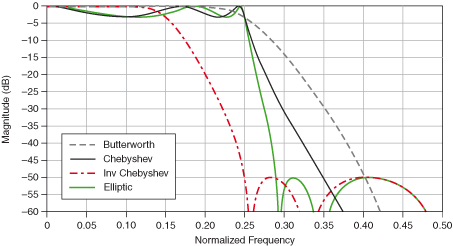
Figure: Examples of filters illustrated here.
Example 1: Filtering a Synthetic Climate Time Series
We build a synthetic daily climate series with three known components: a linear warming trend, a seasonal cycle, and noise. Because we build it ourselves, we know the true components exactly, so we can check how well filtering recovers each one.
We make the noise colored (red) rather than white: real climate noise has more power at low frequencies than at high frequencies. We generate it by shaping the spectrum of white noise in the Fourier domain — scale the amplitude spectrum by , keep random phases, and inverse transform. This choice makes the exercise honest: red noise has power at all frequencies, including the low frequencies where the trend and seasonal cycle live, so no filter can separate the components perfectly.
import numpy as np
import matplotlib.pyplot as plt
from scipy.signal import butter, sosfiltfilt, sosfilt
from scipy.fft import rfft, irfft, rfftfreq

rng = np.random.default_rng(42)

# 10 years of daily data; build t from the sample count so lengths always match
fs = 1.0                     # sampling frequency: 1 sample per day
n = 365 * 10                 # number of samples
time = np.arange(n) / fs     # time in days

# true components
trend = 0.01 * time                          # long-term warming trend, deg C
seasonal = 10 * np.sin(2 * np.pi * time / 365)  # seasonal cycle, period 365 days

# red (colored) noise: shape a white spectrum by 1/f, random phases, inverse FFT
white = rng.standard_normal(n)
freqs = rfftfreq(n, d=1/fs)
shaping = np.zeros_like(freqs)
shaping[1:] = 1 / freqs[1:]      # amplitude ~ 1/f; zero out the mean
noise = irfft(rfft(white) * shaping, n=n)
noise *= 2.5 / np.std(noise)     # scale to a standard deviation of 2.5 deg C

clima = trend + seasonal + noise

# Plot the raw data and the true components
fig, ax = plt.subplots(2, 1, figsize=(10, 6), sharex=True)
ax[0].plot(time, clima, label='Raw data')
ax[0].set_ylabel('Temperature (°C)')
ax[0].set_title('Synthetic climate time series')
ax[0].legend(); ax[0].grid(True)
ax[1].plot(time, trend, label='True trend')
ax[1].plot(time, seasonal, label='True seasonal')
ax[1].plot(time, noise, label='True (red) noise', alpha=0.5)
ax[1].set_xlabel('Time (days)'); ax[1].set_ylabel('Temperature (°C)')
ax[1].legend(); ax[1].grid(True)
plt.show()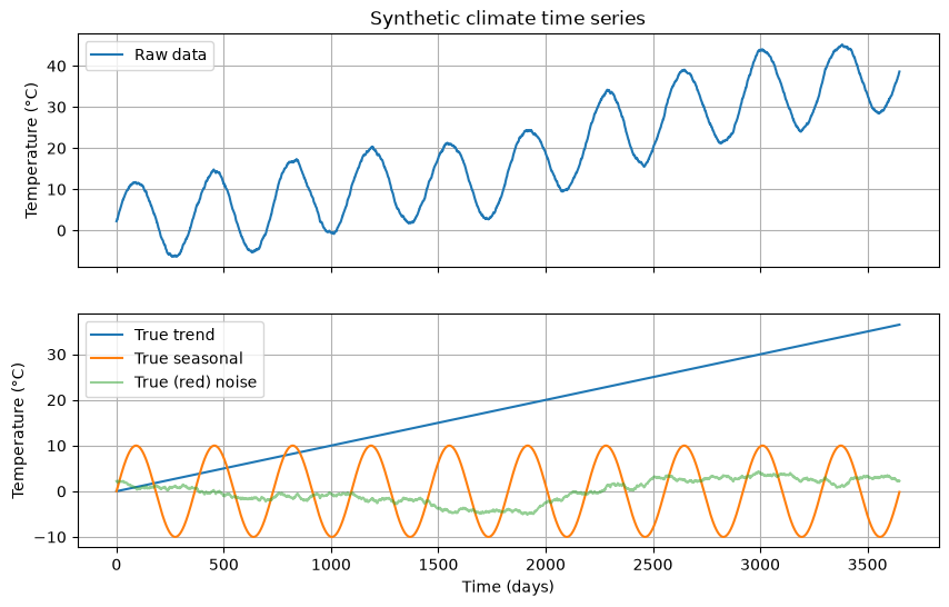
Recovering each component with filters
The three components occupy different frequency bands (frequencies here are in cycles per day):
- the trend lives at very low frequencies, near 0;
- the seasonal cycle is a narrow line at cycles per day;
- the noise spreads across all frequencies.
So we design three Butterworth filters:
- a low-pass with cutoff below the seasonal frequency to recover the trend;
- a band-pass bracketing cycles per day to isolate the seasonal cycle;
- a high-pass with cutoff above the seasonal frequency to isolate the noise.
We use butter(..., output='sos'), which returns the filter as second-order sections: a product of second-order polynomials that represents the same filter but is numerically more stable than the (b, a) polynomial form, especially at high filter orders. We apply the filter with sosfiltfilt, which runs the filter forward and backward so the result has zero phase shift (more on that below).
# Low-pass to recover the trend: cutoff at 1/700 cycles/day, below the seasonal line
sos_lp = butter(4, 1/700, btype='lowpass', fs=fs, output='sos')
clima_trend = sosfiltfilt(sos_lp, clima)

# Band-pass to isolate the seasonal cycle: 1/500 to 1/250 cycles/day brackets 1/365
sos_bp = butter(2, [1/500, 1/250], btype='bandpass', fs=fs, output='sos')
clima_seasonal = sosfiltfilt(sos_bp, clima)

# High-pass to isolate the noise: cutoff at 1/100 cycles/day, above the seasonal line
sos_hp = butter(4, 1/100, btype='highpass', fs=fs, output='sos')
clima_noise = sosfiltfilt(sos_hp, clima)

fig, ax = plt.subplots(3, 1, figsize=(10, 9), sharex=True)
ax[0].plot(time, trend, 'k', label='True trend')
ax[0].plot(time, clima_trend, 'r', label='Low-pass recovered')
ax[0].set_ylabel('°C'); ax[0].set_title('Trend: true vs low-pass filtered')
ax[0].legend(); ax[0].grid(True)

ax[1].plot(time, seasonal, 'k', label='True seasonal')
ax[1].plot(time, clima_seasonal, 'g', label='Band-pass recovered')
ax[1].set_ylabel('°C'); ax[1].set_title('Seasonal cycle: true vs band-pass filtered')
ax[1].legend(); ax[1].grid(True)

ax[2].plot(time, noise, 'k', label='True noise', alpha=0.6)
ax[2].plot(time, clima_noise, 'b', label='High-pass recovered', alpha=0.6)
ax[2].set_xlabel('Time (days)'); ax[2].set_ylabel('°C')
ax[2].set_title('Noise: true vs high-pass filtered')
ax[2].legend(); ax[2].grid(True)
plt.tight_layout()
plt.show()

# quantify the recovery errors
for name, true_c, rec in [('trend', trend, clima_trend),
                          ('seasonal', seasonal, clima_seasonal),
                          ('noise', noise, clima_noise)]:
    rms = np.sqrt(np.mean((true_c - rec)**2))
    print(f"RMS error of recovered {name}: {rms:.2f} °C")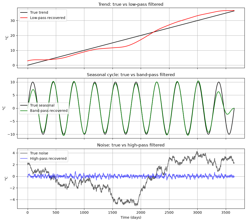
RMS error of recovered trend: 2.45 °C
RMS error of recovered seasonal: 1.55 °C
RMS error of recovered noise: 2.49 °C
Why the recovery is imperfect: spectral leakage between components
The recovered trend is not a straight line: it wanders around the true trend. The recovered noise is missing part of the true noise. This is not a bug in the filters — it is a property of the data.
A filter separates signals by frequency band. It can only separate components cleanly if they occupy disjoint bands. Here the red noise has power at all frequencies, including below the low-pass cutoff. That low-frequency part of the noise passes through the low-pass filter along with the trend, and there is no way for the filter to tell them apart. The same leakage contaminates the band-pass output: the recovered “seasonal” series contains the noise power that falls inside the pass band, so its amplitude fluctuates from year to year even though the true seasonal cycle is perfectly regular. Meanwhile the high-pass output misses the low-frequency part of the noise — and red noise holds most of its power at low frequencies, so the high-pass filter recovers only a small fraction of the true noise and its RMS error is nearly as large as the noise itself.
Also note the filter edges: near the start and end of the series, the filter has incomplete data and the output is distorted. Edge effects are a standard filtering artifact; taper or trim the edges before interpreting them.
The lesson: filtering recovers a frequency band, not a physical component. The two coincide only when the components are spectrally separated. With colored noise, some leakage is unavoidable, and you should report it rather than ignore it.
Zero-phase versus causal filtering
scipy.signal gives two ways to apply an SOS filter:
sosfiltruns the filter forward in time only. This is a causal filter: the output at time depends only on samples up to . This is the only option in real-time systems, and it preserves the onset of a signal — nothing appears in the output before it appears in the input. The cost is a frequency-dependent phase delay: features in the output arrive late.sosfiltfiltruns the filter forward, then backward. The two passes cancel each other’s phase delay, so the output has zero phase: filtered features stay aligned in time with the raw data. The cost is that the filter is no longer causal — energy leaks backward in time, so a sharp onset acquires a small precursor. Use it for offline analysis when timing alignment matters, never for real-time processing, and be careful when picking arrival times near sharp onsets.
We demonstrate the difference on the seismic data below, where the sharp P-wave onset makes the phase delay easy to see.
Use Cases in Geoscience:
- Climate change studies: Filtering temperature data to remove noise and focus on long-term trends.
- El Niño and La Niña detection: Filtering helps identify periodic oscillations in sea surface temperature data.
- Weather forecasting: High-pass filters isolate short-term variations for analysis.
Example 2: Application to Seismology
We download the same data as in lecture 2.8: seismograms recorded in the Puget Sound (station UW.RATT) for the M8.2 Chignik, Alaska earthquake of July 29, 2021, plus a noise window before the event. We query the FDSN data center with the IRIS client; note that IRIS data services are now operated by EarthScope, but the client name IRIS still works.
The channel code HHZ denotes a high-gain broadband seismometer, sampled at 100 samples per second, vertical component. We keep the data in raw digitizer counts here (we do not remove the instrument response), so amplitude axes are labeled in counts.
# Import modules for seismic data
import os

import scipy.signal as signal

# seismic python toolbox
import obspy
import obspy.clients.fdsn.client as fdsn
from obspy import UTCDateTime

os.makedirs('data', exist_ok=True)
# Download seismic data
network = 'UW'
station = 'RATT'
channel = 'HHZ' # broadband high-gain vertical channel, 100 samples per second
Tstart = UTCDateTime(2021, 7, 29, 6, 15)
Tend = Tstart + 7200
fdsn_client = fdsn.Client('IRIS') # client to query the EarthScope (formerly IRIS) DMC server
# call to download the specific data: earthquake waveforms
Z = fdsn_client.get_waveforms(network=network, station=station, location='--', channel=channel,
starttime=Tstart, endtime=Tend)
# basic pre-processing: merge if there are gaps, detrend, taper
Z.merge(); Z.detrend(type='linear'); Z[0].taper(max_percentage=0.05)
# call to download the specific data: noise waveforms (the two hours before the earthquake)
N = fdsn_client.get_waveforms(network=network, station=station, location='--', channel=channel,
starttime=Tstart - 7200, endtime=Tstart)
N.merge(); N.detrend(type='linear'); N[0].taper(max_percentage=0.05)/home/runner/work/mlgeo-book/mlgeo-book/.pixi/envs/default/lib/python3.12/site-packages/obspy/clients/fdsn/client.py:251: ObsPyDeprecationWarning: IRIS is now EarthScope, please consider changing the FDSN client short URL to 'EARTHSCOPE'.
warnings.warn(msg, ObsPyDeprecationWarning)
UW.RATT..HHZ | 2021-07-29T04:15:00.000000Z - 2021-07-29T06:14:59.990000Z | 100.0 Hz, 720000 samplesfig, ax = plt.subplots(2, 1, figsize=(10, 6), sharex=True)
ax[0].plot(Z[0].data); ax[0].grid(True); ax[0].set_ylabel('Counts'); ax[0].set_title('Earthquake window')
ax[1].plot(N[0].data); ax[1].grid(True); ax[1].set_ylabel('Counts'); ax[1].set_title('Noise window')
ax[1].set_xlabel('Sample index')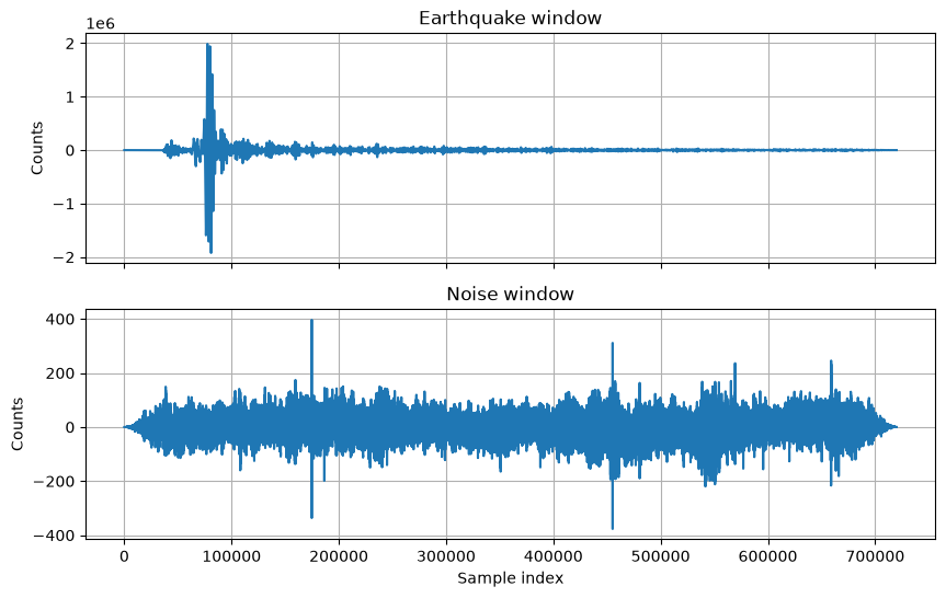
We will use the scipy.signal module to filter the time series.
# sampling rate of the data:
fs = Z[0].stats.sampling_rate
z = np.asarray(Z[0].data)
n_ = np.asarray(N[0].data)

# build the time vector from the number of samples so lengths always match
t = np.arange(len(z)) / fs
We use a butterworth filter of second order, band-passed between the frequencies of 1 Hz and 10 Hz. The sos output is a second-order sections representation: the filter is expressed as a product of second-order polynomials, which is numerically more stable than the single high-order polynomial form. We apply the filter with sosfiltfilt for a zero-phase result.
sos = signal.butter(2, [1, 10], 'bandpass', fs=fs, output='sos')
zf = signal.sosfiltfilt(sos, z)
nf = signal.sosfiltfilt(sos, n_)
fig, axis = plt.subplots(2, 1, figsize=(10, 6), sharex=True)
axis[0].plot(t, zf); axis[0].set_ylabel('Counts'); axis[0].set_title('Earthquake, band-passed 1-10 Hz')
axis[1].plot(t[:len(nf)], nf); axis[1].set_ylabel('Counts'); axis[1].set_title('Noise, band-passed 1-10 Hz')
axis[0].set_xlim([0, 1000]); axis[1].set_xlim([0, 1000])
axis[0].grid(True); axis[1].grid(True)
axis[1].set_xlabel('Time in seconds')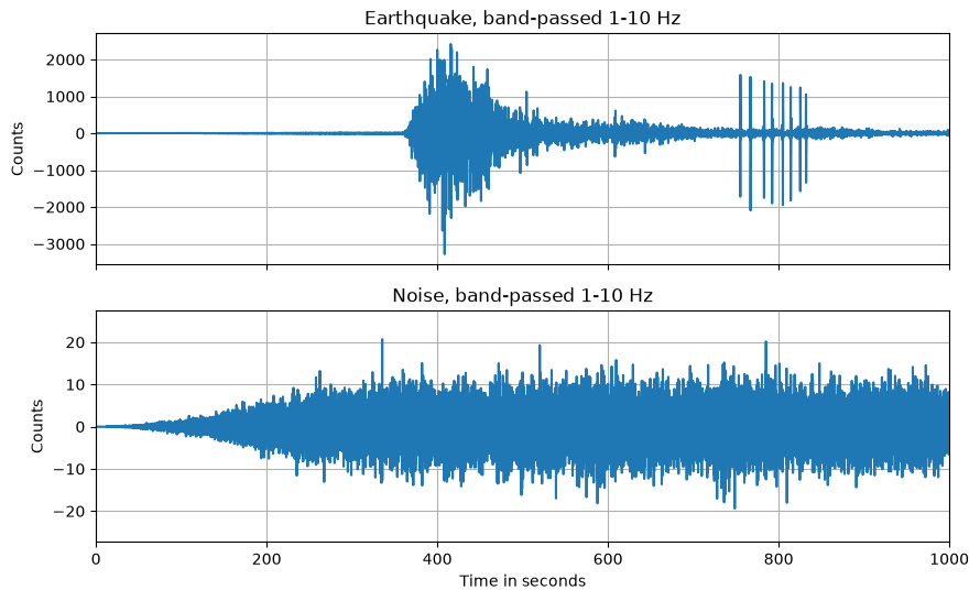
Now filter in a higher frequency band (10-40 Hz) and compare earthquake and noise signals.
sos_hf = signal.butter(2, [10, 40.], 'bandpass', fs=fs, output='sos')
zf_hf = signal.sosfiltfilt(sos_hf, z)
nf_hf = signal.sosfiltfilt(sos_hf, n_)

fig, ax = plt.subplots(2, 1, figsize=(11, 8), sharex=True)
ax[0].plot(t, z); ax[0].plot(t[:len(n_)], n_); ax[0].grid(True)
ax[0].set_title('Raw data'); ax[0].legend(['Earthquake', 'Noise']); ax[0].set_ylabel('Counts')
ax[1].plot(t, zf_hf); ax[1].plot(t[:len(nf_hf)], nf_hf); ax[1].grid(True)
ax[1].set_title('Filtered data, 10-40 Hz'); ax[1].legend(['Earthquake', 'Noise']); ax[1].set_ylabel('Counts')
ax[1].set_xlabel('Time in seconds')
ax[0].set_xlim([700, 1000])
ax[1].set_xlim([700, 1000])
(700.0, 1000.0)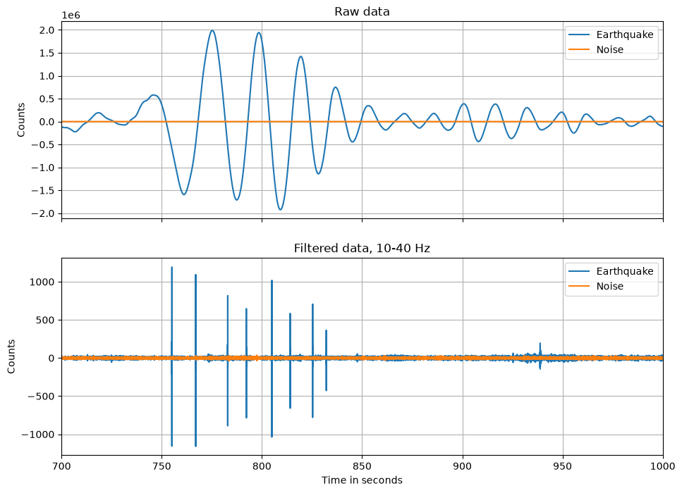
The earthquake stands out from the noise in both frequency bands. In the 10-40 Hz band, the P wave is the dominant arrival: high frequencies attenuate with distance, so the later, slower phases are depleted in high-frequency energy.
Zero-phase (sosfiltfilt) versus causal (sosfilt) filtering
We now apply the same 1-10 Hz band-pass filter both ways and zoom in on the P-wave onset.
zf_zerophase = signal.sosfiltfilt(sos, z)  # forward-backward: zero phase
zf_causal = signal.sosfilt(sos, z)         # forward only: causal, phase-delayed

fig, ax = plt.subplots(2, 1, figsize=(11, 7), sharex=True)
ax[0].plot(t, zf_zerophase, label='sosfiltfilt (zero-phase)')
ax[0].plot(t, zf_causal, label='sosfilt (causal)', alpha=0.8)
ax[0].set_xlim([700, 1000]); ax[0].grid(True); ax[0].legend()
ax[0].set_ylabel('Counts'); ax[0].set_title('Band-passed 1-10 Hz: zero-phase vs causal')

ax[1].plot(t, zf_zerophase, label='sosfiltfilt (zero-phase)')
ax[1].plot(t, zf_causal, label='sosfilt (causal)', alpha=0.8)
ax[1].set_xlim([750, 762]); ax[1].grid(True); ax[1].legend()
ax[1].set_ylabel('Counts'); ax[1].set_xlabel('Time in seconds')
ax[1].set_title('Zoom on the P-wave onset')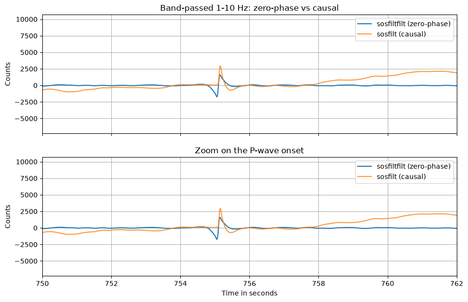
In the zoomed panel, the causal sosfilt output is shifted later in time relative to the zero-phase sosfiltfilt output: the filter’s phase delay moves the apparent onset. The zero-phase version stays aligned with the raw data, but it achieves this by filtering backward in time, which smears a small amount of energy before the onset.
Practical guidance:
- Use causal filtering (
sosfilt) for real-time applications (earthquake early warning) and when the presence or absence of energy before an onset matters. If you pick arrival times on causally filtered data, correct for the filter delay or accept a bias. - Use zero-phase filtering (
sosfiltfilt) for offline analysis where timing alignment between raw and filtered data matters. Do not interpret small precursory wiggles near sharp onsets: they can be filter artifacts.
Example 3: Filtering imperfect records — a gap and a clock error
Everything above assumed a continuous, correctly timed record. Real archives do not oblige: telemetry drops out, disks fill, GPS clocks lose lock. The RATT record happens to be complete and well timed — so we break a copy of it on purpose. That way the unbroken record is the ground truth, and every repair gets graded.
A gap in the record
We knock out 20 seconds of the coda and fill it with zeros, which is how many archives (and a careless merge) deliver dropouts. Then we filter straight across, as if nothing happened.
# Inject a 20 s dropout into the coda, zero-filled
gap_start, gap_end = 850.0, 870.0
i0, i1 = int(gap_start * fs), int(gap_end * fs)
z_gap = z.astype(float).copy()
z_gap[i0:i1] = 0.0

zf_gap = signal.sosfiltfilt(sos, z_gap)  # naive: filter straight across the gap

fig, ax = plt.subplots(2, 1, figsize=(11, 6), sharex=True)
ax[0].plot(t, z_gap, lw=0.8)
ax[0].set_ylabel('Counts'); ax[0].set_title('Raw record with a zero-filled 20 s dropout')
ax[1].plot(t, zf, color='gray', lw=0.8, label='filtered complete record (truth)')
ax[1].plot(t, zf_gap, color='tab:red', lw=0.8, alpha=0.8, label='filtered across the gap')
ax[1].set_ylabel('Counts'); ax[1].set_xlabel('Time in seconds'); ax[1].legend()
for a in ax:
    a.axvspan(gap_start, gap_end, color='k', alpha=0.08)
    a.set_xlim([830, 890]); a.grid(True)
plt.tight_layout()
plt.show()

# Grade against the complete-record reference, by distance from the gap edges
print('distance from gap   local signal RMS   naive filtering error')
for lo, hi in [(0, 2), (2, 5), (5, 10)]:
    w = (((t >= gap_start - hi) & (t < gap_start - lo))
         | ((t >= gap_end + lo) & (t < gap_end + hi)))
    srms = np.sqrt(np.mean(zf[w] ** 2))
    err = np.sqrt(np.mean((zf_gap[w] - zf[w]) ** 2))
    print(f'  {lo}-{hi} s           {srms:7.0f} counts     {err:8.0f} counts '
          f'({err / srms:7.2f}x the signal)')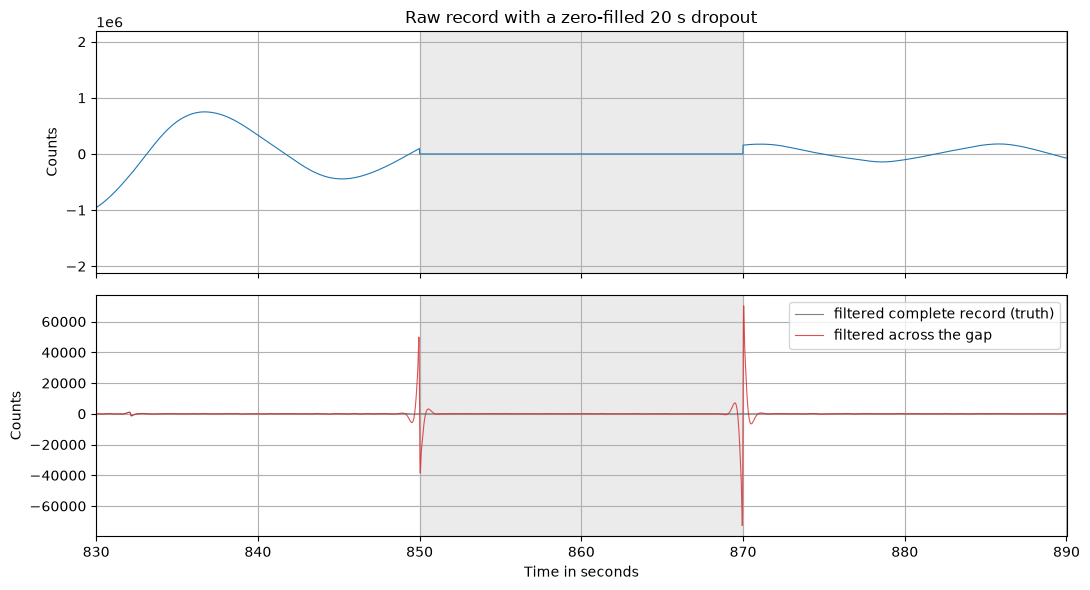
distance from gap   local signal RMS   naive filtering error
  0-2 s                70 counts        12998 counts ( 185.13x the signal)
  2-5 s                74 counts            1 counts (   0.02x the signal)
  5-10 s                62 counts            0 counts (   0.00x the signal)
The damage is out of all proportion to the gap. Zero-filling creates two step discontinuities whose height is the raw amplitude — dominated here by the long-period surface waves, tens of thousands of counts — while the true 1–10 Hz signal in this part of the coda is under a hundred counts. A step is broadband, so the filter responds with its own ringing at the corner frequencies: within two seconds of each edge the output is more than a hundred times the signal, and inside the gap the naive output shows plausible-looking oscillations that are pure filter artifact. As in lesson 2.6, the fabricated samples are the dangerous ones — they look like data.
No filter can resurrect the 20 seconds that were never recorded; repair means confining the damage. The fix is segment-wise filtering: filter each contiguous stretch of real data separately, and leave the gap as NaN. sosfiltfilt pads each segment internally (odd reflection about the endpoints), so no segment ever sees a step.
def filter_with_gaps(x, bad, sos):
    """Zero-phase filter each contiguous valid segment separately.

    The gap itself stays NaN: declared missing, not repaired."""
    out = np.full(len(x), np.nan)
    good_idx = np.flatnonzero(~bad)
    segments = np.split(good_idx, np.flatnonzero(np.diff(good_idx) > 1) + 1)
    for seg in segments:
        out[seg] = signal.sosfiltfilt(sos, x[seg].astype(float))
    return out

bad = np.zeros(len(z), dtype=bool)
bad[i0:i1] = True
zf_seg = filter_with_gaps(z, bad, sos)

fig, ax = plt.subplots(figsize=(11, 4))
ax.plot(t, zf, color='gray', lw=0.8, label='filtered complete record (truth)')
ax.plot(t, zf_seg, color='tab:blue', lw=0.8, alpha=0.8, label='segment-wise filtered')
ax.axvspan(gap_start, gap_end, color='k', alpha=0.08)
ax.set_xlim([830, 890]); ax.grid(True); ax.legend()
ax.set_xlabel('Time in seconds'); ax.set_ylabel('Counts')
ax.set_title('Segment-wise filtering: the gap stays a gap')
plt.tight_layout()
plt.show()

print('distance from gap   naive error         segment-wise error')
for lo, hi in [(0, 2), (2, 5), (5, 10)]:
    w = (((t >= gap_start - hi) & (t < gap_start - lo))
         | ((t >= gap_end + lo) & (t < gap_end + hi)))
    srms = np.sqrt(np.mean(zf[w] ** 2))
    en = np.sqrt(np.mean((zf_gap[w] - zf[w]) ** 2))
    es = np.sqrt(np.nanmean((zf_seg[w] - zf[w]) ** 2))
    print(f'  {lo}-{hi} s          {en / srms:8.2f}x signal    {es / srms:8.4f}x signal')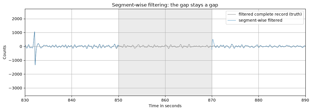
distance from gap   naive error         segment-wise error
  0-2 s            185.13x signal      1.7491x signal
  2-5 s              0.02x signal      0.0005x signal
  5-10 s              0.00x signal      0.0000x signal
Graded against the complete record: segment-wise filtering cuts the near-edge error by two orders of magnitude, and beyond two seconds from the gap it matches the truth to better than a fraction of a percent. The residual contamination spans roughly two seconds — a few periods of the lowest passband frequency (1 Hz), which is the memory of the filter. The practical recipe: filter segments, keep gaps as missing, and flag a guard interval of a few filter periods at each segment edge in your metadata, so downstream users (or your own feature-extraction code in 2.11) know which samples to trust.
A clock error
The second pathology leaves the waveform perfect and corrupts only the timestamps. GPS clock drift, leap-second bugs, and digitizer restarts routinely produce sub-second timing errors — invisible to the eye on any plot, and fatal for phase picks, cross-correlation tomography, and any ML label derived from arrival times. We simulate an instrument whose clock is half a second late, and recover the offset the standard way: cross-correlate against a reference and read the lag of the peak.
offset_true = 0.5  # seconds = 50 samples at 100 Hz
z_late = np.roll(z, int(offset_true * fs))  # same ground motion, stamped 0.5 s late
zf_late = signal.sosfiltfilt(sos, z_late.astype(float))

# Cross-correlate a 60 s window spanning the P arrival
w0, w1 = int(740 * fs), int(800 * fs)
a, b = zf[w0:w1], zf_late[w0:w1]
cc = signal.correlate(b, a, mode='full')
lags = signal.correlation_lags(len(b), len(a), mode='full') / fs
lag_best = lags[np.argmax(cc)]

fig, ax = plt.subplots(2, 1, figsize=(11, 6))
ax[0].plot(t, zf, label='reference clock')
ax[0].plot(t, zf_late, label='faulty clock (+0.5 s)', alpha=0.8)
ax[0].set_xlim([754, 760]); ax[0].grid(True); ax[0].legend()
ax[0].set_ylabel('Counts'); ax[0].set_xlabel('Time in seconds')
ax[0].set_title('The same P wave under two clocks')
ax[1].plot(lags, cc / cc.max())
ax[1].axvline(lag_best, color='r', ls='--', label=f'peak at {lag_best:+.2f} s')
ax[1].set_xlim([-2, 2]); ax[1].grid(True); ax[1].legend()
ax[1].set_xlabel('Lag (s)'); ax[1].set_ylabel('Normalized cross-correlation')
plt.tight_layout()
plt.show()

print(f'injected clock offset:  {offset_true:+.2f} s')
print(f'recovered from the cross-correlation peak: {lag_best:+.2f} s')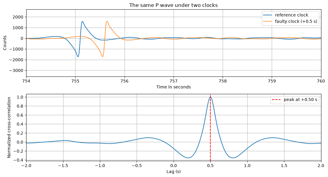
injected clock offset:  +0.50 s
recovered from the cross-correlation peak: +0.50 s
The cross-correlation peak sits at exactly the injected offset: timing errors that no visual inspection would catch are recoverable to the sample, and to a fraction of a sample if you interpolate the correlation peak (fit a parabola through the three points around the maximum). On real data the reference is a co-located sensor, a neighboring station corrected for the predicted travel-time difference, or — for ambient-noise methods — the long-term average of the noise correlation itself, which is how modern networks monitor clock drift continuously. The daily-cadence version of this pathology (a GNSS series reporting the field at the wrong day) is one of the injectable defects in mlgeo_synth.degrade_series, and the repair logic is the same: detect by correlation against a reference, then shift.
Conclusion
Filtering time series data is a routine step in geoscientific analysis. It isolates frequency bands, removes noise, and reveals trends — but it separates bands, not physical components, and every filter choice (corner frequencies, order, causal vs zero-phase) leaves a signature in the output. Know that signature before you interpret the result. And before filtering at all, check the record itself: filter across a zero-filled gap and the artifact will outweigh the signal; trust a timestamp without a reference and a half-second error will ride silently into every product downstream.