2.7 Statistical Considerations for Geoscientific Data and Noise

Canonical Distributions in Geoscientific Data¶

Normal Distribution: Used for variables like temperature, sea level variations, or wind speeds where values are symmetrically distributed around a mean.
Log-Normal Distribution: Observed in phenomena where values cannot be negative and show long tails, such as rainfall intensity, river discharge, grain size, and permeability.
Exponential Distribution: Applied in modeling time intervals between events, such as the time between earthquakes. Earthquake magnitudes follow a related exponential form, the Gutenberg-Richter law, which we work through below.
Power-Law Distribution: Seen in rare, large-scale events like landslides and wildfires, where small events are common and large events are rare.

🖥️ Lecture slides — Session 07 (Wed Oct 14)

1. Statistical Features¶

Let $P(z)$ be the distribution of the data $z$ .

The mean¶

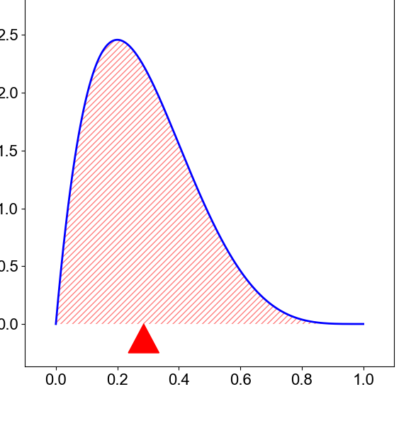
Image taken from this blog.

The mean is the sum of the values divided by the number of data points. It is the first raw moment of a distribution. $\mu = \int_{-\infty}^\infty zP(z)dz$ , where $z$ is the data value (bin) and $P(z)$ is the distribution of the data.

The Variance¶

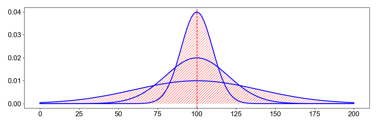
The variance is the second centralized moment. Centralized means that the distribution is shifted around the mean. It calculates how spread out a distribution is.

$\sigma^2 = \int_{-\infty}^\infty (z-\mu)^2P(z)dz$

The standard deviation is the square root of the variance, σ. A high variance indicates a wide distribution.

The skewness¶

Skewness is the third standardized moment. The standardized moment is scaled by the standard deviation. It measures the relative size of the two tails of the distribution.

$m_3= \int_{-\infty}^\infty \frac{(z - \mu)^3}{\sigma^3}P(z)dz$

With the cubic exponent, it is possible that the skewness is negative.

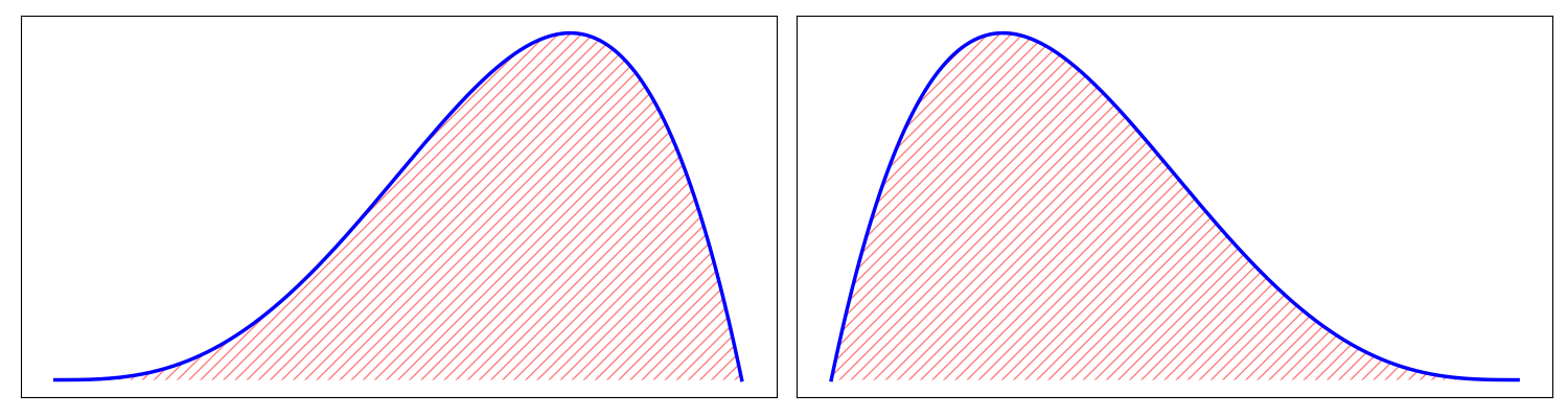
Image taken from this blog.

A positively skewed distribution is one where most of the weight is at the end of the distribution. A negatively skewed distribution is one where most of the weight is at the beginning of the distribution.

Kurtosis¶

Kurtosis measures the combined size of the two tails relative to the whole distribution. It is the fourth centralized and standardized moment.

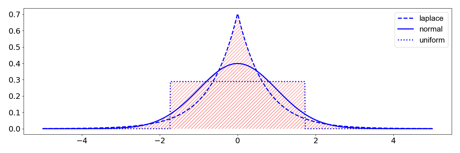$m_4= \int_{-\infty}^\infty (\frac{z-\mu}{\sigma})^4P(z)dz$

The Laplace, normal, and uniform distributions shown all have a mean of 0 and a variance of 1, but their excess kurtosis is 3, 0, and -1.2.

Python functions to calculate the moments might be:

# Import modules
import numpy as np
import matplotlib.pyplot as plt
import pandas as pd
import scipy
import scipy.stats as st
import mlgeo_synth

# One random generator for the whole notebook, seeded for reproducibility.
rng = np.random.default_rng(42)

def raw_moment(X, k, c=0):
    return ((X - c)**k).mean()


def central_moment(X, k):
    return raw_moment(X=X, k=k, c=X.mean())

2. Geological data sets [Level 1]¶

We explore the composition of granite in terms of silica and magnesium content. The data was collected from the EarthChem database.

# Load .csv data into a pandas dataframe
url = 'https://raw.githubusercontent.com/UW-MLGEO/MLGeo-dataset/main/data/EarthRocGranites.csv'
df = pd.read_csv(url)
df.head()

Data pre-processing is often necessary, and most importantly, it is critical to record any processing step applied to raw data. Do not change the original data file; instead, record processing steps. Below, we drop the rows with NaNs (not a number).

df = df.dropna()    # remove rows with NaN values
df.head()

Pandas includes methods to report basic data statistics. Use the describe method of the DataFrame.

df.describe()

# Now, let's visualize the histograms of silica and magnesium

# Create a subplot with two histograms side by side
fig, axes = plt.subplots(1, 2, figsize=(10, 4))  # 1 row, 2 columns

# Plot the histograms for each column
axes[0].hist(df['SIO2(WT%)'], bins=60, color='black')
axes[0].set_xlabel('SiO$_2$, wt%')
axes[0].set_ylabel('Count')
axes[0].set_xlim([40, 100])

axes[1].hist(df['MGO(WT%)'], bins=100, color='black')
axes[1].set_xlabel('MgO, wt%')
axes[1].set_ylabel('Count')
# Note these xlims -> the data largely [but not completely!] sit between 0 and 10 wt%
axes[1].set_xlim([0, 10])

# Add spacing between subplots
plt.tight_layout()
plt.show()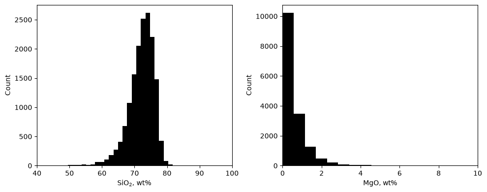

# One more plot: a scatter of SiO2 vs. MgO
plt.scatter(df['SIO2(WT%)'], df['MGO(WT%)'], c='red', alpha=0.125)
ax = plt.gca()
ax.set_xlim([0, 100])
ax.set_xlabel('SiO$_2$, wt%')
ax.set_ylim([0, 100])
ax.set_ylabel('MgO, wt%')
ax.set_aspect('equal')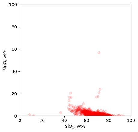

Now, let’s compute the moments for SiO₂ using the functions we defined above.

# The mean:
print(f'The mean is: {raw_moment(df["SIO2(WT%)"], 1):4.2f}')

# Variance:
print(f'The variance is: {central_moment(df["SIO2(WT%)"], 2):4.2f}')

# Skewness:
skewness = central_moment(df["SIO2(WT%)"], 3) / central_moment(df["SIO2(WT%)"], 2) ** (3/2)
print(f'The skewness is: {skewness:4.2f}')

# Kurtosis:
kurtosis_value = central_moment(df['SIO2(WT%)'], 4) / central_moment(df['SIO2(WT%)'], 2) ** 2
print(f'The kurtosis is: {kurtosis_value:4.2f}')

The mean is: 72.11
The variance is: 16.84
The skewness is: -1.75
The kurtosis is: 13.67

# We can also just use pandas (or numpy or scipy):
print('The mean is: %4.2f, the variance is: %4.2f, the skewness is: %4.2f, and the kurtosis is: %4.2f'
      % (df['SIO2(WT%)'].mean(), df['SIO2(WT%)'].var(), df['SIO2(WT%)'].skew(), df['SIO2(WT%)'].kurtosis()))

The mean is: 72.11, the variance is: 16.84, the skewness is: -1.75, and the kurtosis is: 10.67

Note that pandas reports excess kurtosis (normal distribution = 0), while our central_moment version reports plain kurtosis (normal distribution = 3). Keep track of which convention a library uses.

3. Geoscientific distributions¶

Example 1: Sampling from the Normal Distribution

Application: simulate daily temperature variations at a specific location over time. This is a synthetic stand-in, not observations: we draw from a normal distribution with parameters plausible for Seattle (annual mean around 11.5 C, standard deviation around 6 C). Real temperature data have seasonal structure that a single normal distribution does not capture.

# Synthetic stand-in for daily mean temperature in Seattle.
# These are NOT observations; the parameters are plausible values for Seattle.
mean_temp = 11.5  # annual mean temperature (C), plausible for Seattle
std_temp = 6.0    # standard deviation (C), plausible for Seattle

temperatures = rng.normal(loc=mean_temp, scale=std_temp, size=1000)

plt.hist(temperatures, bins=30, color='skyblue', edgecolor='black')
plt.title('Synthetic Temperature Distribution (Normal, Seattle-like parameters)')
plt.xlabel('Temperature (C)')
plt.ylabel('Frequency')
plt.show()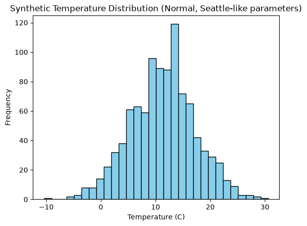

Example 2: Earthquake magnitudes and the Gutenberg-Richter law

Earthquake magnitudes do not follow a log-normal distribution. They follow the Gutenberg-Richter law: the number of earthquakes $N$ with magnitude at least $M$ satisfies

$\log_{10} N = a - bM$ ,

where $a$ sets the overall rate of seismicity and $b$ (the “b-value”) sets the relative rate of small versus large events. Globally, $b \approx 1$ : for each unit drop in magnitude there are about ten times more earthquakes. Because magnitude is already a logarithmic measure of size, this law means earthquake magnitudes follow an exponential distribution above the catalog’s minimum magnitude.

We generate a synthetic catalog with mlgeo_synth.gutenberg_richter_magnitudes, which draws magnitudes with a known b-value.

b_true = 1.0
m_min = 1.0
magnitudes = mlgeo_synth.gutenberg_richter_magnitudes(n=20000, b=b_true, m_min=m_min,
                                                      m_max=8.0, seed=42)
print(f'{len(magnitudes)} magnitudes between {magnitudes.min():.2f} and {magnitudes.max():.2f}')

20000 magnitudes between 1.00 and 5.64

Plot the frequency-magnitude distribution. With the count axis on a log scale, the Gutenberg-Richter law appears as a straight line of slope $-b$ : both the counts per magnitude bin and the cumulative counts $N(\geq M)$ fall off log-linearly.

bins = np.arange(1.0, 8.1, 0.1)
counts, edges = np.histogram(magnitudes, bins=bins)
bin_centers = 0.5 * (edges[:-1] + edges[1:])

# Cumulative count of events with magnitude >= M
mags_sorted = np.sort(magnitudes)
n_cum = len(magnitudes) - np.arange(len(magnitudes))

fig, ax = plt.subplots(figsize=(7, 5))
ax.semilogy(bin_centers[counts > 0], counts[counts > 0], 'ks', ms=4,
            label='counts per 0.1 bin')
ax.semilogy(mags_sorted, n_cum, 'r-', lw=2, label=r'cumulative $N(\geq M)$')
ax.set_xlabel('Magnitude M')
ax.set_ylabel('Number of earthquakes (log scale)')
ax.set_title('Frequency-magnitude distribution (Gutenberg-Richter)')
ax.legend()
ax.grid(True, which='both', alpha=0.3)
plt.show()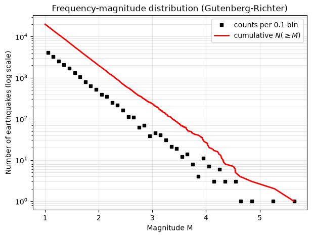

The straight line on the log-scaled count axis is the signature of the Gutenberg-Richter law.

We can estimate the b-value from the data with the maximum-likelihood estimator (Aki 1965):

$\hat{b} = \dfrac{\log_{10}(e)}{\bar{M} - M_{min}}$ ,

where $\bar{M}$ is the mean magnitude of the catalog and $M_{min}$ is the minimum magnitude of completeness.

b_est = np.log10(np.e) / (np.mean(magnitudes) - m_min)
print(f'Maximum-likelihood b-value estimate: {b_est:.3f} (true value: {b_true})')

Maximum-likelihood b-value estimate: 0.998 (true value: 1.0)

The estimate recovers the b-value we put in. On real catalogs, the same estimator works once you have identified the magnitude of completeness (the magnitude above which the network detects every event); below it, the catalog misses small earthquakes and the line bends over.

Example 3: Power-Law Distributions

Application in geosciences: power-law distributions are observed in natural hazard occurrences like landslides and wildfires, where small events are common but large events are rare.

# Generating samples from a power-law distribution
a = 2.5  # Shape parameter (the larger, the steeper the fall-off)
size = 1000

power_law_data = (rng.pareto(a, size) + 1) * 10  # Shifted Pareto distribution

plt.hist(power_law_data, bins=50, color='red', edgecolor='black', log=True)
plt.title('Simulated Data from Power-Law Distribution')
plt.xlabel('Event Size')
plt.ylabel('Frequency (log scale)')
plt.show()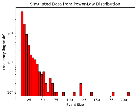

The power-law distribution captures the tail-heavy behavior typical of geophysical processes like landslides.

4. In-class exercise¶

Pick one of the distributions from this lesson, draw samples from it, compute the first four moments, and compare them with the theoretical values. Follow the steps in the cell below.

# In-class exercise: moments of a distribution.
#
# Step 1: pick a distribution and draw 5000 samples with the generator, e.g. one of:
#   samples = rng.normal(loc=11.5, scale=6.0, size=5000)
#   samples = mlgeo_synth.gutenberg_richter_magnitudes(n=5000, b=1.0, m_min=1.0, seed=42)
#   samples = (rng.pareto(2.5, 5000) + 1) * 10
#
# Step 2: compute the first four moments with the functions from Section 1:
#   mean     -> raw_moment(samples, 1)
#   variance -> central_moment(samples, 2)
#   skewness -> central_moment(samples, 3) / central_moment(samples, 2)**(3/2)
#   kurtosis -> central_moment(samples, 4) / central_moment(samples, 2)**2
#
# Step 3: compare with the theoretical values.
#   Normal(mu, sigma): mean mu, variance sigma^2, skewness 0, kurtosis 3.
#   Exponential (Gutenberg-Richter above m_min, rate beta = b*ln(10)):
#     mean m_min + 1/beta, variance 1/beta^2, skewness 2, kurtosis 9.
#
# Step 4: cross-check with scipy: st.skew(samples), st.kurtosis(samples, fisher=False).
#
# Step 5: repeat with only 100 samples. Which moments are most sensitive
#         to sample size, and why?