Before any modeling, you need to know what is in your table. This lesson walks through a standard preparation pipeline on a pandas DataFrame: read the data, inspect types and summary statistics, handle missing values, decide what to do with zeros, and explore correlations and per-class distributions.
The dataset is a synthetic whole-rock geochemistry survey generated by the course package mlgeo_synth. Each row is one rock sample with:
- Major-element oxides (SIO2, AL2O3, FEO, MGO, CAO, NA2O, K2O) in weight percent (wt%),
- density_g_cm3: bulk density in g/cm3,
- mag_susc_si: magnetic susceptibility (SI units),
- label: the lithology (granite, basalt, andesite), which a classifier would later try to predict.
The generator plants realistic correlations: a latent differentiation index drives the oxides, so SiO2 anticorrelates with FeO, MgO, and CaO, and density tracks the mafic oxides. Your job in this lesson is to recover those relationships from the table.
1. Read and Explore the Data
import pandas as pd
import numpy as np
import mlgeo_synth

df = mlgeo_synth.geochem_table(n=10000, seed=42)
df.head()# what datatypes are in the dataset
df.info()<class 'pandas.DataFrame'>
RangeIndex: 10000 entries, 0 to 9999
Data columns (total 10 columns):
# Column Non-Null Count Dtype
--- ------ -------------- -----
0 SIO2 10000 non-null float64
1 AL2O3 10000 non-null float64
2 FEO 10000 non-null float64
3 MGO 10000 non-null float64
4 CAO 10000 non-null float64
5 NA2O 10000 non-null float64
6 K2O 10000 non-null float64
7 density_g_cm3 10000 non-null float64
8 mag_susc_si 10000 non-null float64
9 label 10000 non-null str
dtypes: float64(9), str(1)
memory usage: 847.3 KB
The column label holds strings, everything else is numeric. Check the summary statistics next. Read the min and max rows against physical expectations: oxides should sit between 0 and 100 wt%, and crustal rock densities between roughly 2.5 and 3.3 g/cm3.
# Summary statistics
df.describe()# How many samples per lithology?
df['label'].value_counts()label
granite 5525
basalt 3490
andesite 985
Name: count, dtype: int64The classes are imbalanced: granites outnumber andesites by more than five to one. Keep that number in mind; it comes back in the exercise.
2. Handling Missing Values (NaNs)
Field and lab datasets have gaps: a sensor fails, a lab skips an analysis, a value is dropped during transcription. In pandas, missing values appear as NaN or the newer pd.NA. Common strategies:
- Remove rows/columns with missing values: fine when the missing fraction is small and missingness is unrelated to the value itself.
- Impute: fill gaps with a mean, median, interpolation, or a model-based estimate. Imputation keeps sample size but injects assumptions.
This synthetic table comes out of the generator complete, which real data never is. To give the lesson something to clean, we deliberately knock out a small random fraction of the density and magnetic susceptibility measurements, and we set a few density values to 0 to mimic an instrument that writes 0 when a measurement fails. This kind of “sentinel” zero is common in real archives.
# Deliberately introduce missing data (this is the simulation of a messy archive)
rng = np.random.default_rng(42)

# 2% of density and 3% of susceptibility go missing
mask_density = rng.random(len(df)) < 0.02
mask_susc = rng.random(len(df)) < 0.03
df.loc[mask_density, 'density_g_cm3'] = pd.NA
df.loc[mask_susc, 'mag_susc_si'] = pd.NA

# 15 sentinel zeros in density: the "instrument failure" code
sentinel_rows = rng.choice(len(df), size=15, replace=False)
df.loc[df.index[sentinel_rows], 'density_g_cm3'] = 0.0
# Check for missing values
print(df.isna().sum())SIO2 0
AL2O3 0
FEO 0
MGO 0
CAO 0
NA2O 0
K2O 0
density_g_cm3 187
mag_susc_si 302
label 0
dtype: int64
Note the modern pandas style used above: we assign with df.loc[mask, col] = value and reassign results (df = df.something()) instead of using inplace=True on views or slices. Chained inplace operations on a slice of a DataFrame raise errors in pandas 3.
3. Zeros: Physical Value or Missing-Data Code?
A tempting shortcut is “replace all zeros with NA”. Do not do this. Whether a zero is real depends on the physics of the variable:
- MgO near 0 wt% is real. Highly evolved granites can have essentially no magnesium left; the melt has fractionated it out. The same goes for FeO, CaO, and K2O in the right rock types. Deleting those zeros would preferentially delete evolved granites and bias the dataset.
- A density of 0 g/cm3 is impossible. No rock has zero density. A zero there is a sentinel: a code some instrument or database used to mean “no measurement”.
The check is simple: count zeros per column and ask, for each column, whether zero is inside the physically possible range.
# Count zeros per numeric column
numeric_cols = df.select_dtypes(include='number').columns
print((df[numeric_cols] == 0).sum())
SIO2 0
AL2O3 0
FEO 184
MGO 1434
CAO 367
NA2O 0
K2O 824
density_g_cm3 15
mag_susc_si 0
dtype: int64
Thousands of oxide zeros, and exactly the 15 density zeros we planted. Now look at which rocks carry the MgO zeros.
# Which lithologies have MgO exactly at 0?
print(df.loc[df['MGO'] == 0, 'label'].value_counts())
print("\nMedian SiO2 of MgO=0 samples:", round(df.loc[df['MGO'] == 0, 'SIO2'].median(), 1), "wt%")
print("Median SiO2 of the full table:", round(df['SIO2'].median(), 1), "wt%")
label
granite 1432
andesite 2
Name: count, dtype: int64
Median SiO2 of MgO=0 samples: 74.2 wt%
Median SiO2 of the full table: 69.2 wt%
The MgO zeros are almost all granites, and they are silica-rich ones. That is exactly the geochemical expectation for evolved melts: these zeros carry information. We keep them.
The density zeros are a different story. Replace only those with pd.NA, by assignment, not inplace.
# Convert only the impossible zeros (density) to missing values
df = df.replace({'density_g_cm3': {0.0: pd.NA}})
print(df.isna().sum())
print("\ndensity dtype after replace:", df['density_g_cm3'].dtype)
SIO2 0
AL2O3 0
FEO 0
MGO 0
CAO 0
NA2O 0
K2O 0
density_g_cm3 202
mag_susc_si 302
label 0
dtype: int64
density dtype after replace: object
Look at the dtype: replace with pd.NA silently upcast the column from float64 to object. That matters, because every select_dtypes(include='number') call downstream — the correlation matrices, describe() — would silently drop density, the very column this cleaning was protecting. A column can be numeric in content and non-numeric in dtype, and pandas will not warn you. Cast it back before moving on, and make dtype checks part of every cleaning step, not just the first one.
# Cast back to float so density stays numeric downstream
df['density_g_cm3'] = pd.to_numeric(df['density_g_cm3'])
print("density dtype after cast:", df['density_g_cm3'].dtype)
density dtype after cast: float64
4. Dropping the Incomplete Rows
The missing fraction is small (about 5% of rows have at least one gap) and, by construction here, unrelated to the values themselves, so dropping is defensible. With real data you would first ask why values are missing before dropping anything.
df_cleaned = df.dropna()
print(f"Rows before: {len(df)}, after dropping incomplete rows: {len(df_cleaned)}")
df_cleaned.info()
Rows before: 10000, after dropping incomplete rows: 9499
<class 'pandas.DataFrame'>
Index: 9499 entries, 0 to 9999
Data columns (total 10 columns):
# Column Non-Null Count Dtype
--- ------ -------------- -----
0 SIO2 9499 non-null float64
1 AL2O3 9499 non-null float64
2 FEO 9499 non-null float64
3 MGO 9499 non-null float64
4 CAO 9499 non-null float64
5 NA2O 9499 non-null float64
6 K2O 9499 non-null float64
7 density_g_cm3 9499 non-null float64
8 mag_susc_si 9499 non-null float64
9 label 9499 non-null str
dtypes: float64(9), str(1)
memory usage: 880.1 KB
# Final check: no missing values, class counts still imbalanced but intact
print(df_cleaned.isna().sum())
print()
print(df_cleaned['label'].value_counts())
SIO2 0
AL2O3 0
FEO 0
MGO 0
CAO 0
NA2O 0
K2O 0
density_g_cm3 0
mag_susc_si 0
label 0
dtype: int64
label
granite 5182
basalt 3357
andesite 960
Name: count, dtype: int64
5. Censored Values: Present but Wrong
Missing values announce themselves — isna() finds them. A censored value does not: the instrument reports a number, and the number is wrong in a systematic way. The classic case is a detection limit: a sensor with a reporting floor writes the floor itself whenever the true value falls below it. Geochemical analyses do this (“<0.01 wt%” becomes 0.01), stream gauges do it at low flow, and positioning systems do it near their resolution.
The geochemistry table has no censoring, so we borrow a sensor stream to see the signature. mlgeo_synth.degrade_series injects a detection limit into a synthetic GNSS displacement series and hands back the uncensored truth, so we can measure exactly what censoring does to a statistic.
import matplotlib.pyplot as plt

# A 4-year GNSS displacement series moving at 12 mm/yr, reported by a
# sensor that cannot resolve displacements below 5 mm
gnss = mlgeo_synth.gnss_series(n_years=4, velocity_mm_yr=12.0, seed=7)
censored, truth = mlgeo_synth.degrade_series(gnss, detection_limit_mm=5.0, seed=7)

t = np.arange(len(censored)) / 365.25  # time in years

fig, ax = plt.subplots(1, 2, figsize=(12, 3.8))
ax[0].plot(t, truth['clean'], lw=0.5, color='gray', label='true (uncensored)')
ax[0].plot(t, censored['disp_mm'], lw=0.5, color='tab:red', label='reported')
ax[0].axhline(5.0, color='k', ls='--', lw=1, label='detection limit')
ax[0].set_xlabel('time (yr)'); ax[0].set_ylabel('displacement (mm)')
ax[0].legend()
ax[1].hist(censored['disp_mm'][:365], bins=40, color='tab:red', alpha=0.6, label='reported, year 1')
ax[1].hist(truth['clean'][:365], bins=40, histtype='step', color='gray', label='true, year 1')
ax[1].set_xlabel('displacement (mm)'); ax[1].set_ylabel('count')
ax[1].legend()
plt.tight_layout()
plt.show()

print(f"fraction of samples censored: {censored['censored'].mean():.3f}")
print(f"trend fit on reported values:   {np.polyfit(t, censored['disp_mm'], 1)[0]:.2f} mm/yr")
print(f"trend fit on uncensored values: {np.polyfit(t, truth['clean'], 1)[0]:.2f} mm/yr")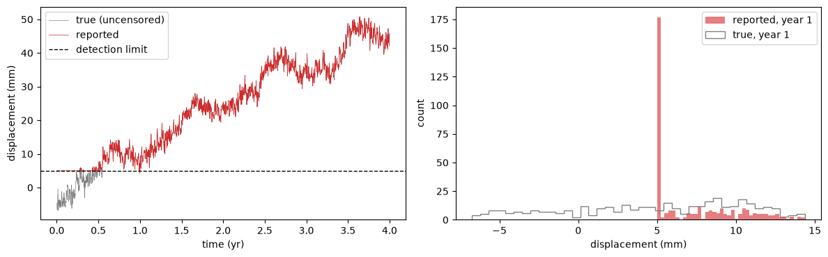
fraction of samples censored: 0.120
trend fit on reported values:   11.59 mm/yr
trend fit on uncensored values: 12.44 mm/yr
Three signatures to remember. First, isna() reports zero missing values: censored data passes every missingness check. Second, the histogram has a heap of identical values exactly at the limit — a spike at a suspiciously round number is the fingerprint of censoring (just as the density zeros were the fingerprint of a sentinel code). Third, statistics are biased in a predictable direction: the reported first-year mean is too high, and the fitted trend is too low, because every low excursion was pulled up to the floor. Dropping the censored samples does not fix this — it removes exactly the low values, which is a worse bias. The honest options are to model the censoring (survival/tobit methods) or to report the limit alongside the data, as lesson 2.13’s data card requires.
A related trap is the mid-record instrument change: a new sensor with a lower detection limit, or a relocated gauge, changes the statistics of the record without any change in the physics. A step in a record’s variance or minimum value is a question for the station metadata before it is a scientific result.
Informative missingness
Section 4 dropped rows on the argument that the gaps were “unrelated to the values themselves” — true here by construction, because we planted them at random (the statisticians’ term is missing completely at random, MCAR). Real instruments rarely oblige. The stream gauge drowns during the flood it was supposed to measure; the GNSS antenna goes silent under the winter storm’s snow load; the field crew skips the site when the road washes out. In each case the value is missing because of the value that would have been measured (missing not at random, MNAR), and dropping those rows systematically deletes the extremes — the floods, the storms — that the analysis probably cares most about. The MgO zeros earlier in this lesson were the same idea in reverse: the “suspicious” values were concentrated in evolved granites, so removing them would have rewritten the geology. Before dropping or imputing anything, ask what process created the gap. If the answer involves the measured quantity, the missingness is itself data, and it belongs in the missing-data policy of your data card.
6. Correlation Analysis
Correlations between features tell you which measurements carry redundant information and hint at the physics behind the table. We compute two matrices:
- Pearson correlation measures linear relationships.
- Spearman rank correlation measures monotonic relationships. It is robust to outliers and to nonlinear but monotonic links, which are common in geochemistry.
The label column is a string, so first keep only the numeric columns.
df_numerical = df_cleaned.select_dtypes(include='number')
df_numerical.head()import seaborn as sns
import matplotlib.pyplot as plt
corr_matrix = df_numerical.corr()
plt.figure(figsize=(10, 8))
sns.heatmap(corr_matrix, annot=True, fmt='.2f', cmap='coolwarm', vmin=-1, vmax=1)
plt.title('Pearson correlation')
plt.tight_layout()
plt.show()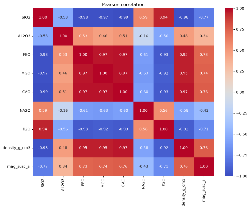
spearman_corr_matrix = df_numerical.corr(method='spearman')

plt.figure(figsize=(10, 8))
sns.heatmap(spearman_corr_matrix, annot=True, fmt='.2f', cmap='coolwarm', vmin=-1, vmax=1)
plt.title('Spearman rank correlation')
plt.tight_layout()
plt.show()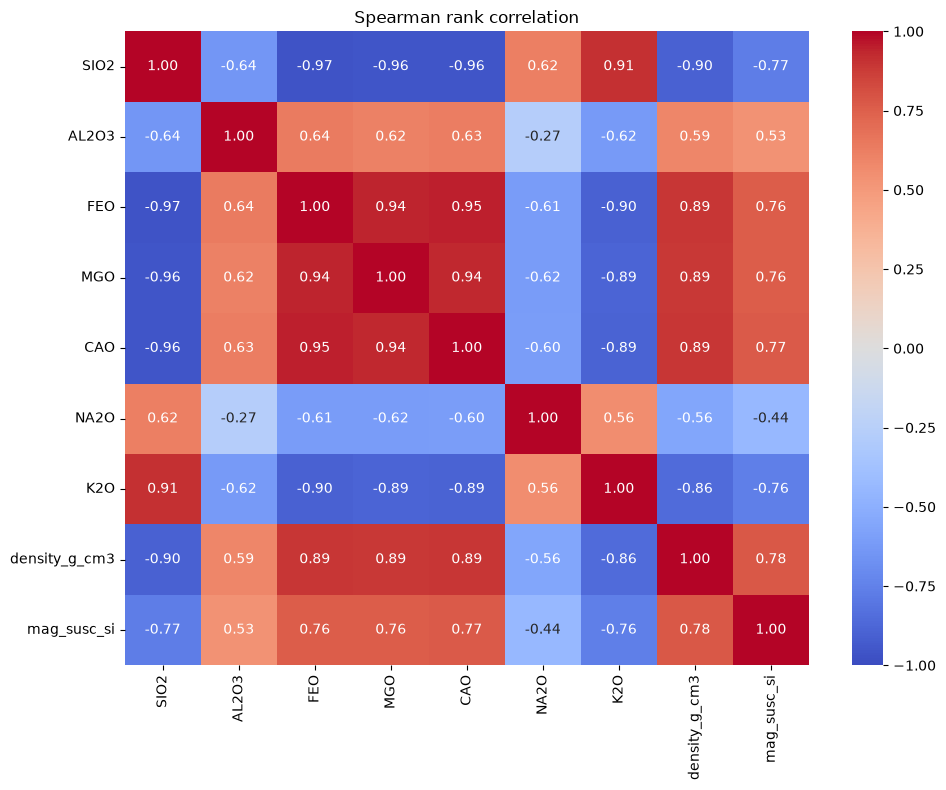
Read the two matrices side by side. SiO2 is strongly anticorrelated with FeO, MgO, and CaO, and positively correlated with K2O. Density tracks the mafic oxides and anticorrelates with SiO2. Where the Spearman value is noticeably stronger than the Pearson value, the relationship is monotonic but not linear; magnetic susceptibility is a typical case, since it spans orders of magnitude.
One structural reason for the negative correlations: oxide analyses are compositional data. The wt% values of the major oxides sum to roughly 100, so if one oxide goes up, the others must come down. This closure effect builds negative correlation into the table regardless of any petrology. Keep it in mind before interpreting every negative entry as a geological process.
7. Feature Distributions per Lithology
Correlation matrices pool all classes together. To see which features separate the lithologies, plot each feature’s distribution per class.
granite = df_cleaned[df_cleaned['label'] == 'granite']
basalt = df_cleaned[df_cleaned['label'] == 'basalt']
andesite = df_cleaned[df_cleaned['label'] == 'andesite']

features = ['SIO2', 'AL2O3', 'FEO', 'MGO', 'CAO', 'NA2O', 'K2O', 'density_g_cm3', 'mag_susc_si']

fig, axes = plt.subplots(3, 3, figsize=(15, 12))
for ax, feature in zip(axes.ravel(), features):
    sns.histplot(granite[feature], kde=True, color='tab:orange', label='granite', stat='density', ax=ax)
    sns.histplot(basalt[feature], kde=True, color='tab:blue', label='basalt', stat='density', ax=ax)
    sns.histplot(andesite[feature], kde=True, color='tab:green', label='andesite', stat='density', ax=ax)
    ax.set_title(feature)
    ax.legend()
plt.tight_layout()
plt.show()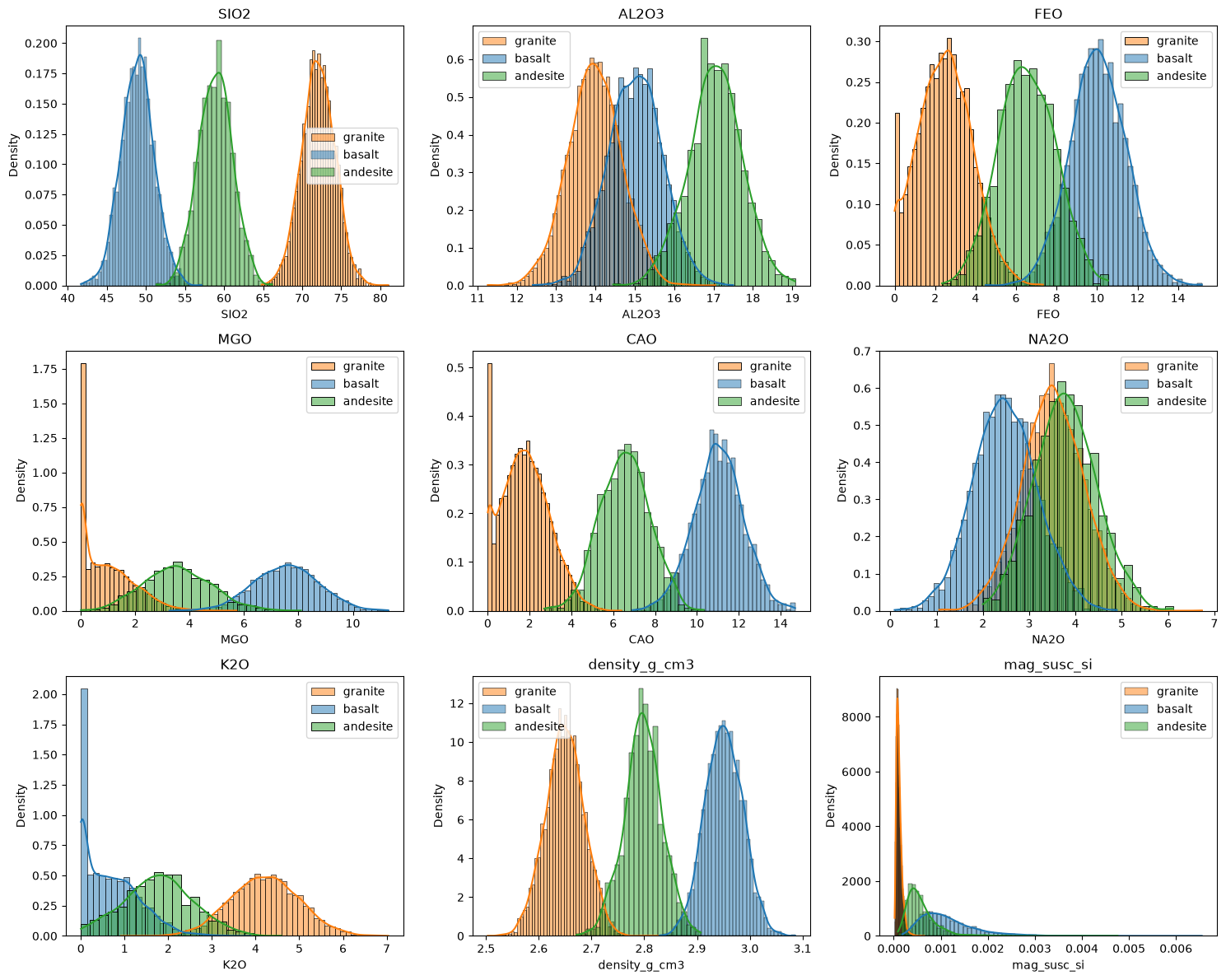
# Boxplots give a compact per-class view of the same information
fig, axes = plt.subplots(3, 3, figsize=(15, 12))
for ax, feature in zip(axes.ravel(), features):
    sns.boxplot(data=df_cleaned, x='label', y=feature, hue='label', ax=ax)
    ax.set_title(feature)
    ax.set_xlabel('')
plt.tight_layout()
plt.show()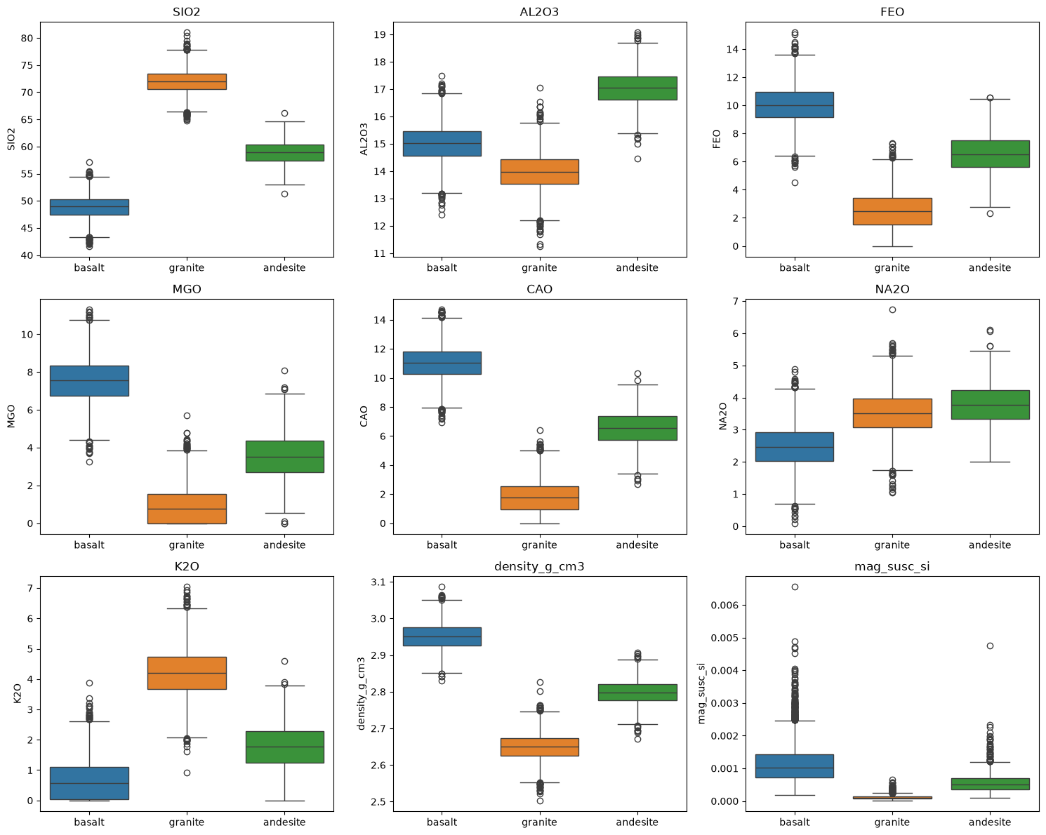
Some features separate the classes almost completely; others overlap heavily. Some distributions look roughly Gaussian, others are skewed or heavy-tailed. To quantify shape, compute skewness and kurtosis alongside the usual moments.
from scipy.stats import skew, kurtosis

def summarize_distribution(frame, features):
    summary = {}
    for feature in features:
        values = frame[feature].to_numpy(dtype=float)
        summary[feature] = {
            'mean': values.mean(),
            'median': np.median(values),
            'std': values.std(),
            'skewness': skew(values),
            'kurtosis': kurtosis(values),
        }
    return pd.DataFrame(summary)

print("Granite:")
print(summarize_distribution(granite, features).round(3))
print("\nBasalt:")
print(summarize_distribution(basalt, features).round(3))
print("\nAndesite:")
print(summarize_distribution(andesite, features).round(3))
Granite:
SIO2 AL2O3 FEO MGO CAO NA2O K2O density_g_cm3 \
mean 72.043 13.981 2.481 0.947 1.799 3.511 4.213 2.650
median 72.040 13.977 2.477 0.756 1.753 3.503 4.210 2.649
std 2.128 0.677 1.319 0.930 1.129 0.672 0.785 0.037
skewness -0.007 -0.001 0.180 0.880 0.332 -0.003 0.033 -0.006
kurtosis 0.015 0.121 -0.326 0.191 -0.370 0.061 -0.067 0.058
mag_susc_si
mean 0.000
median 0.000
std 0.000
skewness 1.796
kurtosis 5.938
Basalt:
SIO2 AL2O3 FEO MGO CAO NA2O K2O density_g_cm3 \
mean 48.931 15.014 10.044 7.547 11.032 2.479 0.677 2.951
median 48.976 15.028 10.029 7.564 11.025 2.470 0.571 2.951
std 2.121 0.681 1.367 1.187 1.187 0.690 0.631 0.036
skewness 0.001 -0.002 0.017 -0.031 -0.038 0.053 0.854 0.023
kurtosis 0.083 0.001 0.087 -0.040 0.079 -0.025 0.352 -0.105
mag_susc_si
mean 0.001
median 0.001
std 0.001
skewness 1.616
kurtosis 4.949
Andesite:
SIO2 AL2O3 FEO MGO CAO NA2O K2O density_g_cm3 \
mean 58.910 17.041 6.544 3.545 6.553 3.779 1.775 2.798
median 58.943 17.050 6.519 3.504 6.565 3.761 1.780 2.798
std 2.142 0.681 1.381 1.227 1.169 0.668 0.791 0.036
skewness -0.009 -0.093 0.044 0.155 -0.063 0.117 0.061 -0.062
kurtosis -0.132 0.117 -0.235 -0.032 -0.089 -0.085 -0.206 0.151
mag_susc_si
mean 0.001
median 0.000
std 0.000
skewness 3.393
kurtosis 27.926
Skewness near 0 and kurtosis near 0 (scipy uses the excess-kurtosis convention) indicate a roughly Gaussian shape. Large positive skewness, as in magnetic susceptibility, signals a heavy right tail; such features are often log-transformed before modeling.
Save the cleaned table for later chapters.
df_cleaned.to_csv('cleaned_geochem.csv', index=False)
df_cleaned.describe()8. Exercise
Answer with code and a short written justification for each question.
- Correlations and closure. From the Pearson matrix, list the three strongest anticorrelations with SiO2. How much of that anticorrelation is petrology (mafic minerals fractionating out as melts evolve) and how much is the closure effect (major oxides summing to ~100 wt%, so one rising forces others down)? Propose one check that could help separate the two explanations.
- Best separating feature. Using the per-class histograms and the summary statistics, which single feature best separates the three lithologies? Support your choice quantitatively, for example by comparing the difference in class means to the class standard deviations for each feature.
- Class imbalance. Granites make up more than half the table and andesites about 10%. If you trained a classifier on this table and measured only overall accuracy, what accuracy would a model that always predicts “granite” achieve? What does that imply about how you should evaluate a future classifier on this dataset?
- Zeros revisited. Suppose a colleague hands you a version of this table where all MgO zeros were already replaced with NaN and dropped. Which class would lose the most samples, and how would the SiO2 distribution of the remaining granites change?
# your answers here