1. Introduction
Feature engineering is the process of transforming raw data into quantities — features — that can be used in statistical analysis and prediction.
Key types of features include:
Statistical features
Statistical features summarize the distribution of data values: central tendency, dispersion, and shape.
- Mean: average value of the data points.
- Variance/Standard Deviation: measure of the spread of the data.
- Skewness: asymmetry in the distribution of values.
- Kurtosis: “tailedness” of the distribution.
- Percentiles: threshold values for different segments of the distribution.
Temporal features
Temporal features describe the time-dependent patterns within a series.
- Autocorrelation: correlation of a time series with a lagged version of itself.
- Trend: long-term increase or decrease in the data.
- Seasonality: regular patterns that repeat over a specific period.
- Change points: locations where the statistical properties of the series change.
Below we build a synthetic daily series with a trend and a yearly cycle, remove the trend, and measure the lag-1 autocorrelation of what remains.
import numpy as np
import pandas as pd
import matplotlib.pyplot as plt

rng = np.random.default_rng(42)

# Create a 3-year daily time series with trend and seasonality
t = np.arange(0, 365 * 3)
seasonal_series = rng.standard_normal(3 * 365) + np.linspace(0, 10, 3 * 365) + \
    2 * np.sin(2 * np.pi * np.linspace(0, 3, 3 * 365))

# fit a trend using least squares regression
slope, intercept = np.polyfit(t, seasonal_series, 1)
trend = slope * t + intercept
# the seasonal component is what remains after removing the trend
seasonal = seasonal_series - trend
# lag-1 autocorrelation of the detrended series
autocorr_seasonal = np.corrcoef(seasonal[:-1], seasonal[1:])[0, 1]
print(f'Lag-1 autocorrelation of the detrended seasonal series: {autocorr_seasonal:.2f}')

# Plot the original time series, trend, and seasonal component
plt.figure(figsize=(10, 6))
plt.plot(seasonal_series, label='Original Time Series')
plt.plot(trend, label='Trend')
plt.plot(seasonal, label='Seasonal (detrended)')
plt.xlabel('Day')
plt.legend()
Lag-1 autocorrelation of the detrended seasonal series: 0.68
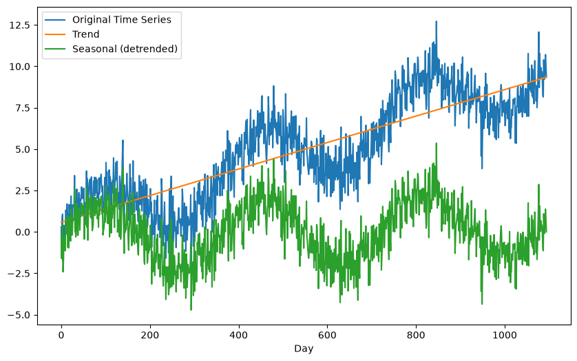
The detrended series still carries the yearly cycle, so neighboring days are similar and the lag-1 autocorrelation is high. Compare with pure white noise of the same length: white noise has no memory, so its lag-1 autocorrelation is near zero.
white_series = rng.standard_normal(3 * 365)

autocorr_white = np.corrcoef(white_series[:-1], white_series[1:])[0, 1]
print(f'Lag-1 autocorrelation of the detrended seasonal series: {autocorr_seasonal:.2f}')
print(f'Lag-1 autocorrelation of white noise:                   {autocorr_white:.2f}')
Lag-1 autocorrelation of the detrended seasonal series: 0.68
Lag-1 autocorrelation of white noise: -0.00
Spatial features
For geospatial data, spatial features capture the relationships between different locations in an image or dataset.
- Texture: patterns in the local intensity variations (e.g., smooth, rough).
- Spatial correlation: measures how similar nearby locations are in terms of intensity values.
from scipy.ndimage import gaussian_filter
from scipy.fft import fft2, ifft2, fftshift

# Generate a 2D grid (e.g., geospatial data, such as a topographic map)
n = 100  # size of the grid
x = np.linspace(0, 10, n)
y = np.linspace(0, 10, n)
X2d, Y2d = np.meshgrid(x, y)

# 2D white noise
white_noise_2d = rng.standard_normal((n, n))

# Spatially correlated noise: smooth the white noise with a Gaussian filter
spatially_correlated_noise = gaussian_filter(white_noise_2d, sigma=3)

plt.figure(figsize=(12, 6))

plt.subplot(1, 2, 1)
plt.imshow(white_noise_2d, extent=[0, 10, 0, 10], cmap='viridis')
plt.xlabel('x')
plt.ylabel('y')
plt.colorbar(label='Amplitude')
plt.title('2D White Noise')

plt.subplot(1, 2, 2)
plt.imshow(spatially_correlated_noise, extent=[0, 10, 0, 10], cmap='viridis')
plt.xlabel('x')
plt.ylabel('y')
plt.colorbar(label='Amplitude')
plt.title('2D Spatially Correlated Noise')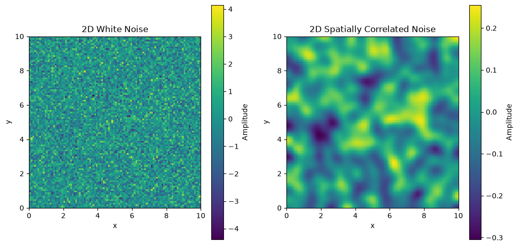
Spatial autocorrelation of the white noise, computed via the power spectrum (Wiener-Khinchin theorem):
# 2D Fourier transform of the white noise
fft_white_noise = fft2(white_noise_2d)

# power spectrum
power_spectrum = np.abs(fft_white_noise) ** 2

# inverse transform of the power spectrum gives the autocorrelation function
autocorrelation_white = np.real(ifft2(power_spectrum))

# shift the zero-lag component to the center
autocorrelation_white = fftshift(autocorrelation_white)

# normalize
autocorrelation_white /= autocorrelation_white.max()
Spatial autocorrelation of the correlated noise:
fft_noise = fft2(spatially_correlated_noise)
power_spectrum = np.abs(fft_noise) ** 2
autocorrelation = np.real(ifft2(power_spectrum))
autocorrelation = fftshift(autocorrelation)
autocorrelation /= autocorrelation.max()
plt.figure(figsize=(11, 6))
# White noise (unfiltered)
plt.subplot(2, 2, 1)
plt.imshow(white_noise_2d, extent=[0, 10, 0, 10], cmap='viridis')
plt.xlabel('x')
plt.ylabel('y')
plt.colorbar(label='Amplitude')
plt.title('2D White Noise')
plt.subplot(2, 2, 2)
plt.imshow(autocorrelation_white, extent=[-5, 5, -5, 5], cmap='viridis')
plt.xlabel('x')
plt.ylabel('y')
plt.colorbar(label='Amplitude')
plt.title('2D White Noise Autocorrelation')
# Spatially correlated noise
plt.subplot(2, 2, 3)
plt.imshow(spatially_correlated_noise, extent=[0, 10, 0, 10], cmap='viridis')
plt.xlabel('x')
plt.ylabel('y')
plt.colorbar(label='Amplitude')
plt.title('2D Spatially Correlated Noise')
plt.subplot(2, 2, 4)
plt.imshow(autocorrelation, extent=[-5, 5, -5, 5], cmap='viridis')
plt.xlabel('x')
plt.ylabel('y')
plt.colorbar(label='Normalized Amplitude')
plt.title('Autocorrelation Function')
plt.tight_layout()
plt.show()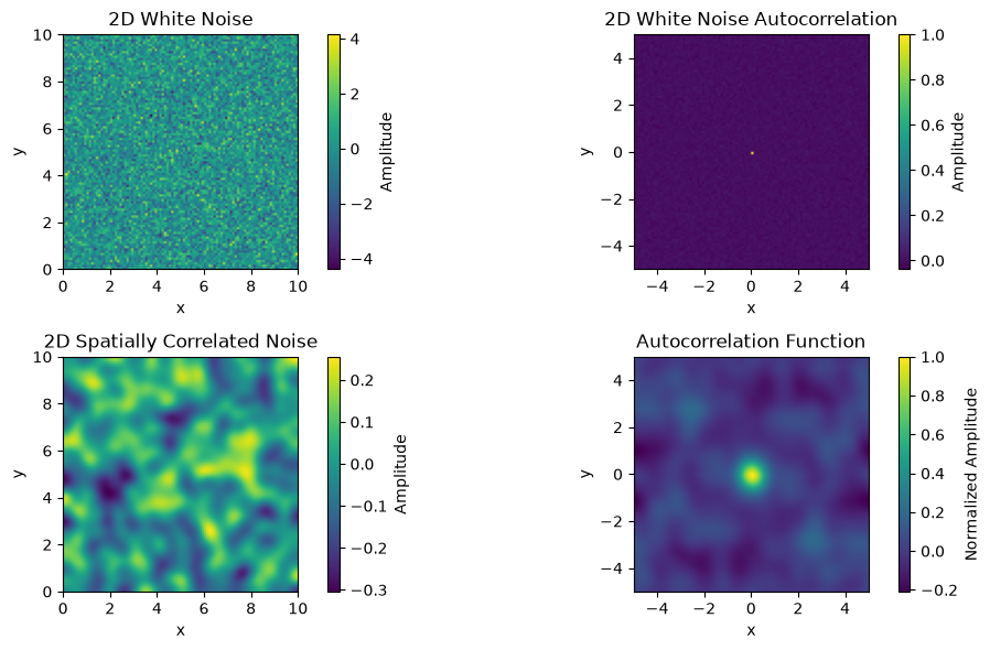
Estimate the feature “correlation length” of the two images. The correlation length is often measured as the distance at which the autocorrelation function decays to 1/e of its maximum value.
center = n // 2
# correlation length for the white noise
autocorr_center = autocorrelation_white[center, center:]
distances = np.linspace(0, 5, center)
correlation_length_white = np.interp(1 / np.e, autocorr_center[::-1], distances[::-1])

# correlation length for the spatially correlated noise
autocorr_center = autocorrelation[center, center:]
correlation_length = np.interp(1 / np.e, autocorr_center[::-1], distances[::-1])

print(f'Estimated correlation length for white noise: {correlation_length_white:.2f} '
      f'and for spatially correlated noise: {correlation_length:.2f}')
Estimated correlation length for white noise: 0.07 and for spatially correlated noise: 0.61
Fractal features
Fractal features describe the self-similarity or complexity of the data across scales. A common one is the fractal dimension: a smooth curve has dimension close to 1, while a rough curve that fills more of the plane has a dimension closer to 2.
The Higuchi method estimates the fractal dimension of a time series. It measures the average “length” of the curve at coarser and coarser subsamplings; the slope of log(length) versus log(scale) gives the dimension.
def higuchi_fd(series, kmax=10):
    """Higuchi fractal dimension of a 1D time series.

    Builds kmax coarse-grained versions of the series, measures the mean
    curve length at each scale k, and fits the slope of
    log(length) vs log(1/k). Returns the estimated fractal dimension,
    between 1 (smooth) and 2 (rough).
    """
    series = np.asarray(series, dtype=float)
    npts = len(series)
    lengths = []
    for k in range(1, kmax + 1):
        lk = []
        for m in range(k):
            idx = np.arange(m, npts, k)
            if len(idx) < 2:
                continue
            dist = np.sum(np.abs(np.diff(series[idx])))
            # normalization factor for the subsampled curve
            norm = (npts - 1) / (len(idx) - 1) / k
            lk.append(dist * norm / k)
        lengths.append(np.mean(lk))
    coeffs = np.polyfit(np.log(1.0 / np.arange(1, kmax + 1)), np.log(lengths), 1)
    return coeffs[0]


print(f'Higuchi fractal dimension of white noise:         '
      f'{higuchi_fd(white_series):.2f}')
print(f'Higuchi fractal dimension of the seasonal series: '
      f'{higuchi_fd(seasonal_series):.2f}')
smooth_series = gaussian_filter(white_series, sigma=5)
print(f'Higuchi fractal dimension of smoothed noise:      '
      f'{higuchi_fd(smooth_series):.2f}')
Higuchi fractal dimension of white noise: 1.99
Higuchi fractal dimension of the seasonal series: 1.98
Higuchi fractal dimension of smoothed noise: 1.10
White noise is maximally rough, so its dimension is near 2. Smoothing lowers the dimension toward 1. The fractal dimension is a single number that captures roughness, which makes it a compact feature for classifying signals.
2. Seismic Time Series Data Example
This section demonstrates how to automatically extract features using a simple Python package, tsfel, applied to seismic waveforms recorded in the Pacific Northwest.
The miniPNW subset includes labeled seismic waveforms for events of various origins:
- Earthquakes
- Explosions (mostly quarry blasts)
- Surface events (such as avalanches and landslides)
- Sonic booms
- Thunder
We will explore how features vary across these classes of seismic events.
Dataset citation. The data is a subset of the PNW-ML benchmark: Ni, Y., Hutko, A., Skene, F., Denolle, M., Malone, S., Bodin, P., Hartog, R., & Wright, A. (2023). Curated Pacific Northwest AI-ready Seismic Dataset. Seismica, 2(1). doi:Ni et al. (2023). The archival access path to the full dataset is seisbench.data.PNW(); here we use a small subset (“miniPNW”) hosted on a class server.
# Import modules for seismic data and feature extraction
import numpy as np
import matplotlib.pyplot as plt
import pandas as pd
import scipy
import scipy.stats as st
import os
import urllib.request
import h5py  # for reading .h5 files
We download two files from the class storage into ./data/: the waveforms as an HDF5 file and their associated metadata as a CSV file. The metadata file is small. The waveform file is large (about 1 GB), so we guard its download: if it fails, the notebook prints a message and skips the waveform-dependent cells.
os.makedirs('data', exist_ok=True)

base_url = 'https://dasway.ess.washington.edu/shared/niyiyu/PNW-ML'
metadata_path = './data/miniPNW_metadata.csv'
waveform_path = './data/miniPNW_waveforms.hdf5'

# metadata: small CSV, always download if missing
if not os.path.exists(metadata_path):
    urllib.request.urlretrieve(f'{base_url}/miniPNW_metadata.csv', metadata_path)
print(f'Metadata file present: {os.path.exists(metadata_path)}')

# waveforms: large HDF5, guarded download
if not os.path.exists(waveform_path):
    try:
        print('Downloading waveform file (large, be patient)...')
        urllib.request.urlretrieve(f'{base_url}/miniPNW_waveforms.hdf5',
                                   waveform_path)
    except Exception as e:
        if os.path.exists(waveform_path):
            os.remove(waveform_path)  # remove partial file
        raise RuntimeError(
            'Could not download miniPNW_waveforms.hdf5 from '
            f'{base_url}. Check your network connection, or place the file '
            'manually in ./data/. Original error: ' + repr(e)) from e
print(f'Waveform file present: {os.path.exists(waveform_path)}')
Metadata file present: True
Downloading waveform file (large, be patient)...
Waveform file present: True
Metadata
We first read the metadata and arrange it into a pandas DataFrame.
df = pd.read_csv(metadata_path)
# Display the first few rows of the DataFrame
df.head()The nature of the event source is stored in one of the metadata attributes.
df['source_type'].unique()<ArrowStringArray>
['earthquake', 'explosion', 'sonic_boom', 'thunder', 'surface_event']
Length: 5, dtype: strAssume that we are exploring features to classify the waveforms into the categories of event types. We take the source_type attribute as the label.
labels = df['source_type']
print(labels.value_counts())
source_type
earthquake 500
explosion 500
surface_event 500
sonic_boom 126
thunder 94
Name: count, dtype: int64
How many seismic waveforms are there in each category?
counts = labels.value_counts()
fractions = counts / counts.sum()
for name, count in counts.items():
    print(f'{name:>15s}: {count:5d} waveforms ({100 * fractions[name]:.1f}%)')
earthquake: 500 waveforms (29.1%)
explosion: 500 waveforms (29.1%)
surface_event: 500 waveforms (29.1%)
sonic_boom: 126 waveforms (7.3%)
thunder: 94 waveforms (5.5%)
Would you say that this is a balanced dataset with respect to the classes of interest? Class imbalance matters: a classifier trained on this set will see many more of the dominant class, and accuracy alone becomes a misleading score.
counts.plot(kind='bar')
plt.ylabel('Number of waveforms')
plt.title('Class balance of the miniPNW dataset')
plt.tight_layout()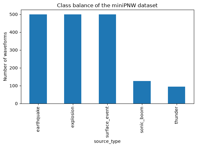
Waveform data
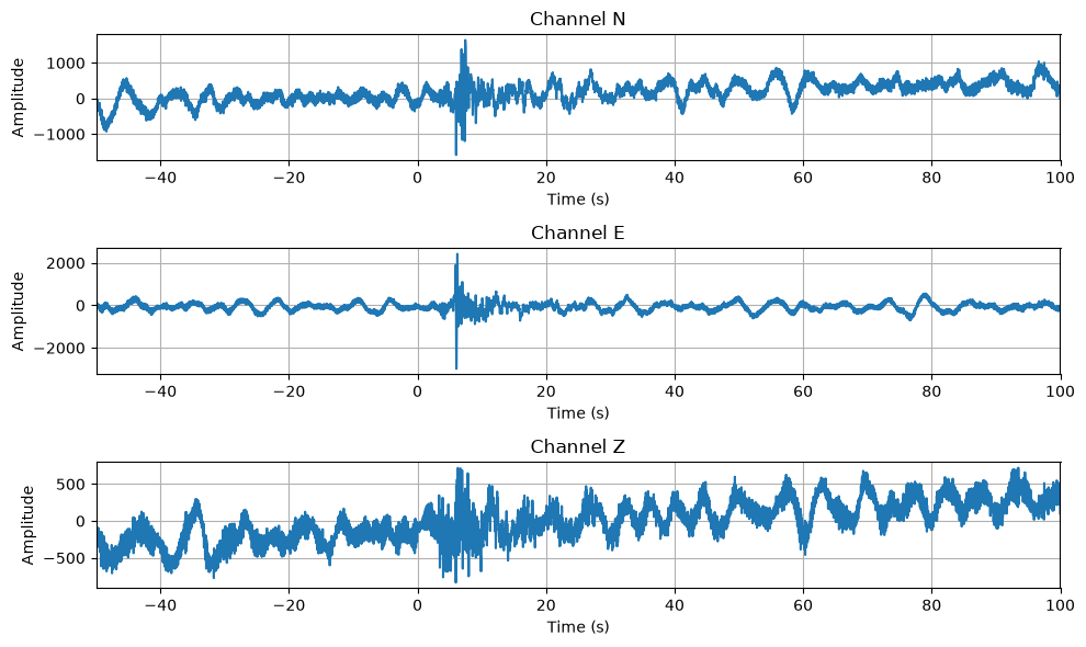
Now we read the waveform data. It is stored in an HDF5 file under a finite number of groups. Each group has an array of datasets that correspond to the waveforms. To link the metadata to the waveform files, the key trace_name has the dataset ID. The address is labeled as follows:
bucketX$i,:3,:nwhere X is the HDF5 group number and i is the index. The file typically has 3 waveforms, one from each direction of ground motion: N, E, Z. In the following, we focus on the vertical (Z) waveforms.
All cells that need the waveform file are gated behind a file-existence check, so the notebook still runs top to bottom if the download failed.
chan_list = ['N', 'E', 'Z']

if os.path.exists(waveform_path):
    f = h5py.File(waveform_path, 'r')
else:
    print('Waveform file not found: skipping waveform cells.')
Below, a function to read a waveform out of the file.
def read_data(tn, f):
    """
    Read the waveform data from the .h5 file.
    tn: trace_name of the waveform
    f: open h5py file object
    """
    bucket, narray = tn.split('$')  # split trace_name into bucket and indices
    x, y, z = [int(i) for i in narray.split(',:')]
    data = f['/data/%s' % bucket][x, :y, :z]  # read the data as a 2D array
    return data
The trace name is stored as a data attribute in the metadata.
trace_names = list(df['trace_name'])
trace_names[0]'bucket1$0,:3,:15001'if os.path.exists(waveform_path):
example_waveform = read_data(trace_names[530], f)
print(f'The first dimension of the data is {example_waveform.shape[0]}')
print(f'The second dimension of the data is {example_waveform.shape[1]}')
# the time vector goes from -50 to 100 s around the pick, at 100 Hz
t = np.linspace(-50, 100, example_waveform.shape[1])
# plot an example of the data in a 3-row subplot
fig, ax = plt.subplots(3, 1, figsize=(10, 6))
for i in range(3):
ax[i].plot(t, example_waveform[i, :])
ax[i].set_title(f'Channel {chan_list[i]}')
ax[i].set_xlabel('Time (s)')
ax[i].set_ylabel('Amplitude')
ax[i].grid(True)
ax[i].set_xlim(-50, 100)
plt.tight_layout()
else:
print('Waveform file not found: skipping waveform plot.')The first dimension of the data is 3
The second dimension of the data is 15001
We extract the Z component of every waveform and stack them into a single array.
if os.path.exists(waveform_path):
    nt = example_waveform.shape[-1]
    ndata = len(labels)
    Z = np.zeros(shape=(ndata, nt))
    for i in range(ndata):
        Z[i, :] = read_data(df.iloc[i]['trace_name'], f)[2, :nt]
    print(f'We have a total of {Z.shape[0]} data samples and each has '
          f'{Z.shape[1]} data points')
else:
    print('Waveform file not found: skipping waveform stacking.')
We have a total of 1720 data samples and each has 15001 data points
Automatic feature extraction with tsfel
Now we have data and its attributes, in particular the label as source type. We are going to extract features automatically with tsfel and explore how they vary across classes.
tsfel organizes features by domain (statistical, temporal, spectral). We load the default configuration:
import tsfel

cfg = tsfel.get_features_by_domain()
print(list(cfg.keys()))
/home/runner/work/mlgeo-book/mlgeo-book/.pixi/envs/default/lib/python3.12/site-packages/tsfel/feature_extraction/calc_features.py:195: SyntaxWarning: invalid escape sequence '\*'
\**kwargs:
['spectral', 'statistical', 'temporal', 'fractal']
tsfel takes a 1D array and the sampling rate, and returns a one-row DataFrame of features. We wrap the extraction into a function that loops over a set of waveforms, attaches the label, and cleans up the column names (tsfel prefixes every column with 0_).
Note on runtime: extracting the full feature set for every waveform in miniPNW takes too long for class. We cap the extraction to a random subset of about 200 waveforms. Feel free to raise the cap outside of class.
def calculate_features(Z, indices, df, cfg, fs=100.0):
    """
    Calculate tsfel features for a subset of waveforms.
    Z: 2D array of seismic data (n_waveforms, n_samples)
    indices: which rows of Z to process
    df: metadata DataFrame (for the source_type label)
    cfg: tsfel feature configuration

    Returns:
    X: DataFrame of features, one row per waveform, with a source_type column
    """
    rows = []
    for count, i in enumerate(indices):
        if count % 20 == 0:
            print(f'Extracting features from sample {count}/{len(indices)}')
        Xi = tsfel.time_series_features_extractor(cfg, Z[i, :], fs=fs, verbose=0)
        Xi['source_type'] = df.iloc[i]['source_type']
        rows.append(Xi)
    X = pd.concat(rows, axis=0, ignore_index=True)
    # remove the 0_ prefix that tsfel adds to every column name
    X.columns = X.columns.str.removeprefix('0_')
    return X
if os.path.exists(waveform_path):
import time
n_subset = min(200, ndata)
subset_rng = np.random.default_rng(42)
subset_idx = subset_rng.choice(ndata, size=n_subset, replace=False)
start = time.time()
X = calculate_features(Z, subset_idx, df, cfg)
end = time.time()
print(f'Time taken to calculate features for {n_subset} waveforms: '
f'{end - start:.2f} seconds')
else:
print('Waveform file not found: skipping feature extraction.')Extracting features from sample 0/200
Extracting features from sample 20/200
Extracting features from sample 40/200
Extracting features from sample 60/200
Extracting features from sample 80/200
Extracting features from sample 100/200
Extracting features from sample 120/200
Extracting features from sample 140/200
Extracting features from sample 160/200
Extracting features from sample 180/200
Time taken to calculate features for 200 waveforms: 33.51 seconds
if os.path.exists(waveform_path):
    display(X.head())
else:
print('Waveform file not found: no features to show.')New DataFrame clean up
Removing the samples with NaN or infinity.
if os.path.exists(waveform_path):
    print(f'no of samples in the dataframe: {X.shape[0]}')
    # Replace infinities with NaN
    new_X = X.replace([np.inf, -np.inf], np.nan, inplace=False)
    # Drop rows with NaN values
    new_X = new_X.dropna(inplace=False)
    print(f'no of samples in the new dataframe: {new_X.shape[0]}')
else:
    print('Waveform file not found: skipping cleanup.')
no of samples in the dataframe: 200
no of samples in the new dataframe: 200
Explore correlation among features
if os.path.exists(waveform_path):
    import seaborn as sns

    # Compute pairwise correlation of columns
    corr_matrix = new_X.drop('source_type', axis=1).corr().abs()

    # Mask the upper triangle (the matrix is symmetric)
    mask = np.triu(np.ones_like(corr_matrix, dtype=bool))

    plt.figure(figsize=(15, 10))
    sns.heatmap(corr_matrix, mask=mask, cmap='coolwarm', vmax=1, vmin=-1,
                center=0, square=True, linewidths=.5, annot=False)
    plt.show()
else:
    print('Waveform file not found: skipping correlation heatmap.')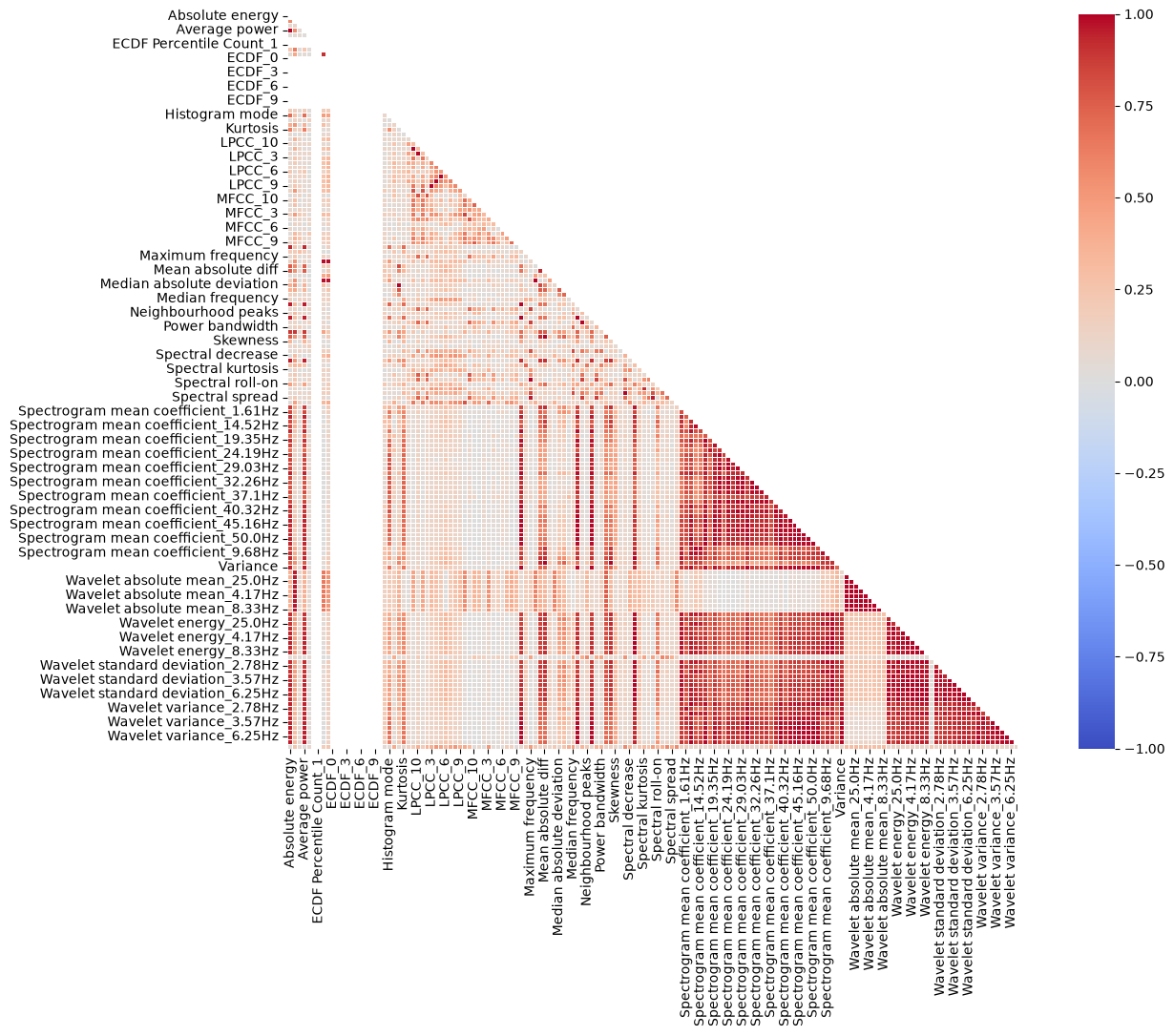
Blocks of highly correlated features are redundant: they carry the same information. Dimensionality reduction (next lesson) or feature selection can prune them.
Exploring the feature space for classification
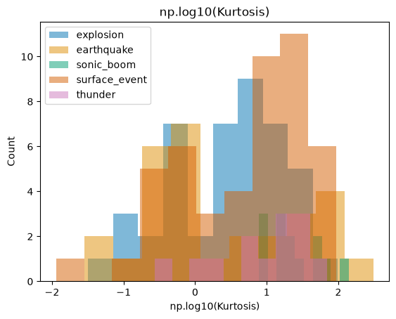
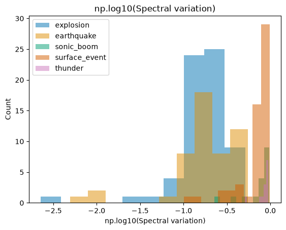
Here we plot distributions of selected features among the classes. A feature is useful for classification when its distributions separate between classes.
def plot_feature_histograms(new_X, feature):
    import seaborn as sns
    # Get unique source types
    source_types = new_X['source_type'].unique()

    # colorblind-friendly palette
    colors = sns.color_palette('colorblind')

    for i, source_type in enumerate(source_types):
        # Select data for this source type
        data = new_X[new_X['source_type'] == source_type][feature]

        # Plot histogram for this source type
        plt.hist(np.log10(data), color=colors[i % len(colors)], alpha=0.5,
                 label=source_type)

    plt.title(f'np.log10({feature})')
    plt.xlabel(f'np.log10({feature})')
    plt.ylabel('Count')
    plt.legend()
    plt.show()
if os.path.exists(waveform_path):
feature = 'Area under the curve'
plot_feature_histograms(new_X, feature)
feature = 'Kurtosis'
plot_feature_histograms(new_X, feature)
feature = 'Spectral variation'
plot_feature_histograms(new_X, feature)
else:
print('Waveform file not found: skipping feature histograms.')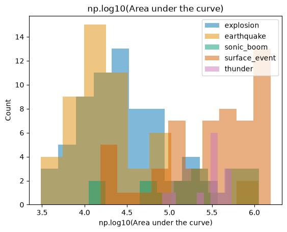
/home/runner/work/mlgeo-book/mlgeo-book/.pixi/envs/default/lib/python3.12/site-packages/pandas/core/arraylike.py:402: RuntimeWarning: invalid value encountered in log10
  result = getattr(ufunc, method)(*inputs, **kwargs)
Student exercise
- Which of the features will be best to classify among the event type classes?
Use the scaffold below. The idea: a feature separates two classes well when the difference between the class means is large compared to the spread within each class. Rank the features by that criterion.
if os.path.exists(waveform_path):
    # Answer scaffold: rank features by class separation.
    # Step 1: group the features by class.
    grouped = new_X.groupby('source_type')

    # Step 2: for each feature, compute the spread of the class means
    #         divided by the mean within-class standard deviation.
    feature_cols = new_X.columns.drop('source_type')
    class_means = grouped[feature_cols].mean()
    class_stds = grouped[feature_cols].std()
    separation = class_means.std(axis=0) / class_stds.mean(axis=0)

    # Step 3: sort and show the 10 most discriminative features.
    top10 = separation.sort_values(ascending=False).head(10)
    print(top10)

    # Step 4 (your turn): plot histograms of the top-ranked features with
    # plot_feature_histograms(new_X, feature) and check the separation by eye.
    # Step 5 (your turn): does the ranking change if you normalize each
    # feature first? Try (new_X - mean) / std before Step 2.
else:
    print('Waveform file not found: skipping student exercise scaffold.')
ECDF_9 inf
ECDF_5 inf
ECDF_6 inf
ECDF_2 inf
ECDF_4 inf
Entropy inf
Spectral variation 2.033088
MFCC_0 1.909093
MFCC_3 1.392157
LPCC_11 1.376106
dtype: float64
Self-check
separationis a Series with one positive value per feature column (156 here);class_meansandclass_stdshave one row per class (5) and one column per feature.- Some entries come out as
inf: those features (severalECDF_*,Entropy) are constant within each class, so the within-class standard deviation is zero. Discard them — a constant feature carries no per-event information. - Among the finite values, spectral features (
Spectral variation,MFCC_*,LPCC_*) rank near the top with separations around 1-2. - Step 4: histograms of top-ranked features show class distributions that only partly overlap; a low-ranked feature shows nearly identical histograms for all classes.
- Step 5: the ranking does not change. Rescaling a feature multiplies the spread of its class means and its within-class spread by the same factor, so their ratio — and therefore the ranking — is unchanged.
- Ni, Y., Hutko, A., Skene, F., Denolle, M., Malone, S., Bodin, P., Hartog, R., & Wright, A. (2023). Curated Pacific Northwest AI-ready Seismic Dataset. Seismica, 2(1). 10.26443/seismica.v2i1.368