This lesson is the capstone of the data pillar. The previous lessons taught you to read, clean, transform, and describe geoscience data. This one defines what it means for a dataset to be AI-ready, and demonstrates the two failure modes that ruin otherwise careful projects: preprocessing leakage and wrong splits for autocorrelated data.

1. An operational definition of AI-ready data
“AI-ready” is not a feeling. A dataset is AI-ready when it passes this checklist:
- Documented provenance, license, and citation. Where did every byte come from, who owns it, and how must it be cited? If part of the data is synthetic, that is disclosed.
- Machine-readable metadata (a data card). A file that ships with the data and states what the variables are, in what units, how they were collected or generated, and what the known limitations are. A README written for humans is not enough; the card should be parseable (YAML, JSON).
- Tidy shapes. One row per observation, one column per variable for tables; explicit, labeled dimensions for arrays. No merged header rows, no units embedded in strings.
- Explicit units. Every physical variable carries its unit in the metadata, not in a comment someone will lose.
- A missing-data policy. Which values are missing, why, how they are encoded (
NaN,pd.NA, a sentinel), and what the recommended handling is. - Benchmark splits shipped with the data. Train/validation/test membership is stored as a column or an index file, so every user evaluates on the same held-out data.
- Leakage controls. The split design respects the correlation structure of the data (time, space, event membership), and all preprocessing statistics are computed from the training split only.
- A class and event inventory. How many samples, how many of each class, how many distinct events. Rare-event problems look very different from balanced ones, and users must know before they train.
The rest of this notebook builds a small dataset that passes the checklist, then breaks rules 6 and 7 on purpose so you can see the damage in the metrics.
2. Workflow reminders: from raw data to an ML dataset
Before the checklist can be satisfied, the data has to exist in a usable form. A condensed workflow, from the earlier lessons:
- Pose the problem in general terms. Transform into ? Predict from ? Choosing a target variable already poses the problem (regression, classification, detection).
- Establish what is realistically possible. Review the literature, ML and not. If experts reach accuracy , that is your first benchmark.
- Compile and organize the data early. One location, machine-readable structures (NumPy, Xarray, pandas), saved in standard formats (Parquet, netCDF, Zarr, HDF5). Never overwrite the raw data.
- Characterize the data. Histograms, distributions, cross-plots, correlation matrices (lessons 2.4 and 2.7). Save the exploration scripts.
- Consider feature extraction and dimensionality reduction. Statistical, temporal, or spectral features (lesson 2.11); PCA or ICA (lesson 2.12).
- Consider augmentation. Bootstrap, synthetic noise, transformed copies — with disclosed provenance (lessons 2.6 and 2.10).
- Make the pipeline reproducible. A script or an sklearn
Pipelinethat goes from raw data to the AI-ready product with no manual steps.
import os

import matplotlib.pyplot as plt
import numpy as np
import pandas as pd

import mlgeo_synth

rng = np.random.default_rng(2026)
os.makedirs("data/ai_ready_demo", exist_ok=True)
3. Build the dataset: a river-discharge-like series with rare floods
We generate ten years of a daily discharge-like series: a seasonal baseflow cycle plus noise, with rare flood events injected as a Poisson process. Because the generator is ours, we know the ground truth: every sample carries a label (event) and an event identifier (event_id). This is exactly the kind of synthetic dataset lesson 2.10 called admissible — we use it to develop and benchmark methodology, and we disclose how it was made.
The task we will pose: nowcast whether today is a flood day from the previous seven days of discharge. Floods are rare, so this is an imbalanced classification problem — common in the geosciences (floods, earthquakes, landslides, algal blooms).
n_years = 10
n_days = int(365.25 * n_years)
day = np.arange(n_days)

# Seasonal baseflow: winter-peaking annual cycle plus white noise, in m^3/s
baseflow = 25.0 + 12.0 * np.cos(2 * np.pi * (day - 20) / 365.25) + rng.normal(0, 3.0, n_days)

df = mlgeo_synth.inject_rare_events(
    baseflow,
    rate_per_year=4.0,
    duration_days=(3, 15),
    amplitude=(5.0, 60.0),
    shape="spike",
    samples_per_day=1,
    seed=2026,
)
df.index = pd.date_range("2015-01-01", periods=len(df), freq="D")
df.index.name = "date"
df = df.rename(columns={"value": "discharge_m3s"})
df.head()fig, ax = plt.subplots(figsize=(11, 3.5))
ax.plot(df.index, df["discharge_m3s"], lw=0.6, color="steelblue", label="discharge")
ax.fill_between(df.index, 0, df["discharge_m3s"].max(), where=df["event"] == 1,
color="firebrick", alpha=0.3, label="flood (label = 1)")
ax.set_xlabel("date")
ax.set_ylabel("discharge (m$^3$/s)")
ax.legend(loc="upper right")
ax.set_title("Synthetic daily discharge with injected rare floods")
plt.tight_layout()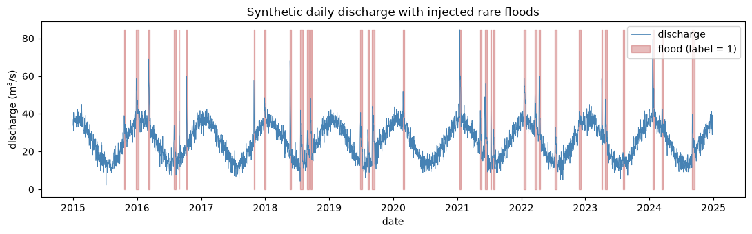
# Zoom on one event to see the shape: sharp rise, exponential recession
one_event = df[df["event_id"] == df.loc[df["event"] == 1, "event_id"].iloc[0]]
window = df.loc[one_event.index[0] - pd.Timedelta(days=15):
                one_event.index[-1] + pd.Timedelta(days=25)]
fig, ax = plt.subplots(figsize=(8, 3))
ax.plot(window.index, window["discharge_m3s"], color="steelblue")
ax.fill_between(window.index, 0, window["discharge_m3s"].max(),
                where=window["event"] == 1, color="firebrick", alpha=0.3)
ax.set_ylabel("discharge (m$^3$/s)")
ax.set_title("One flood event (shaded)")
plt.tight_layout()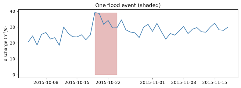
The class and event inventory
Checklist item 8. Two different numbers matter and they are not interchangeable: the fraction of samples that are labeled 1, and the number of distinct events. Cross-validation folds are counted in events, not samples: 40 events split five ways leaves only ~8 events per fold, no matter how many flood-days there are.
n_events = df.loc[df["event_id"] >= 0, "event_id"].nunique()
durations = df[df["event_id"] >= 0].groupby("event_id").size()

inventory = pd.Series({
    "total samples (days)": len(df),
    "flood samples": int(df["event"].sum()),
    "flood sample fraction": round(df["event"].mean(), 4),
    "distinct flood events": n_events,
    "median event duration (days)": durations.median(),
    "max event duration (days)": int(durations.max()),
})
inventory
total samples (days) 3652.0000
flood samples 312.0000
flood sample fraction 0.0854
distinct flood events 33.0000
median event duration (days) 9.0000
max event duration (days) 15.0000
dtype: float644. The data card
Checklist items 1, 2, 4, 5, and 8, in one machine-readable file. A data card travels with the data — same folder, same repository, versioned together. Below is the card for this dataset, in YAML:
name: synthetic_discharge_floods
version: "1.0"
created: "2026-08-11"
description: >
  Ten years of synthetic daily river-discharge-like data with rare injected
  flood events, for teaching rare-event classification and split design.
provenance:
  synthetic: true                      # disclosed, per lesson 2.10
  generator: mlgeo_synth.inject_rare_events
  generator_params: {rate_per_year: 4.0, duration_days: [3, 15],
                     amplitude: [5.0, 60.0], shape: spike, seed: 2026}
  background: "25 + 12*cos(annual cycle) + N(0, 3.0), seed 2026"
license: CC-BY-4.0
citation: "MLGeo course materials, University of Washington, 2026 edition."
sampling:
  cadence: daily
  start: "2015-01-01"
  n_samples: 3652
variables:
  discharge_m3s: {dtype: float64, units: m^3/s, description: daily mean discharge}
  event:         {dtype: int64, units: null, description: "label: 1 = flood day"}
  event_id:      {dtype: int64, units: null, description: "flood id; -1 = background"}
  split:         {dtype: str, values: [train, val, test], description: benchmark split}
missing_data:
  policy: "no missing values by construction; real gauges gap during floods —
           document gaps, do not silently interpolate labels"
class_inventory:
  flood_sample_fraction: ~0.09
  distinct_events: ~40
splits:
  scheme: chronological
  train: "2015-01-01 to 2021-12-31"
  val:   "2022-01-01 to 2022-12-31"
  test:  "2023-01-01 to 2024-12-31"
  rule: "no event spans a split boundary check; preprocessing statistics
         from train only"
known_limitations:
  - synthetic; event shapes are idealized (linear rise, exponential decay)
  - no measurement gaps, rating-curve errors, or sensor drift
Nothing here is decoration. Every entry answers a question a future user (including future you) would otherwise have to guess about.
# Ship the splits WITH the data (checklist item 6): a split column, assigned
# chronologically, then write data + card to the same folder.
df["split"] = "train"
df.loc["2022-01-01":"2022-12-31", "split"] = "val"
df.loc["2023-01-01":, "split"] = "test"
print(df["split"].value_counts())
print("\nFlood events per split:")
print(df[df["event_id"] >= 0].groupby("split", observed=True)["event_id"].nunique())
split
train 2557
test 730
val 365
Name: count, dtype: int64
Flood events per split:
split
test 6
train 22
val 5
Name: event_id, dtype: int64
data_card = """\
name: synthetic_discharge_floods
version: "1.0"
created: "2026-08-11"
description: >
  Ten years of synthetic daily river-discharge-like data with rare injected
  flood events, for teaching rare-event classification and split design.
provenance:
  synthetic: true
  generator: mlgeo_synth.inject_rare_events
  generator_params: {rate_per_year: 4.0, duration_days: [3, 15], amplitude: [5.0, 60.0], shape: spike, seed: 2026}
license: CC-BY-4.0
citation: "MLGeo course materials, University of Washington, 2026 edition."
sampling: {cadence: daily, start: "2015-01-01", n_samples: %d}
variables:
  discharge_m3s: {dtype: float64, units: m^3/s}
  event: {dtype: int64, description: "label: 1 = flood day"}
  event_id: {dtype: int64, description: "flood id; -1 = background"}
  split: {dtype: str, values: [train, val, test]}
missing_data: {policy: "no missing values by construction"}
splits: {scheme: chronological, train: "2015-2021", val: "2022", test: "2023-2024"}
""" % len(df)

df.to_csv("data/ai_ready_demo/synthetic_discharge_floods.csv")
with open("data/ai_ready_demo/data_card.yml", "w") as f:
    f.write(data_card)
sorted(os.listdir("data/ai_ready_demo"))
['data_card.yml', 'synthetic_discharge_floods.csv']# "Machine-readable" means a script can consume it. Read the card back:
import yaml
with open("data/ai_ready_demo/data_card.yml") as f:
card = yaml.safe_load(f)
print(card["variables"]["discharge_m3s"])
print(card["splits"]){'dtype': 'float64', 'units': 'm^3/s'}
{'scheme': 'chronological', 'train': '2015-2021', 'val': '2022', 'test': '2023-2024'}
5. Features for a flood classifier
We build a deliberately simple feature set: the discharge on each of the previous seven days (lag features, q_lag1 = yesterday through q_lag7), plus the annual cycle encoded as sine and cosine of day-of-year. Today’s discharge is not a feature — using it would make the task trivial (a flood day is a high-discharge day). Nowcasting from the past keeps the problem honest and keeps the label out of the features. The point of this lesson is not the model — it is what the splits and the preprocessing do to the evaluation.
feat = pd.DataFrame(index=df.index)
for lag in range(1, 8):
    feat[f"q_lag{lag}"] = df["discharge_m3s"].shift(lag)
doy = df.index.dayofyear
feat["doy_sin"] = np.sin(2 * np.pi * doy / 365.25)
feat["doy_cos"] = np.cos(2 * np.pi * doy / 365.25)
feat["event"] = df["event"]
feat["event_id"] = df["event_id"]
feat["split"] = df["split"]
feat = feat.dropna()

X = feat[[c for c in feat.columns if c.startswith(("q_lag", "doy_"))]]
y = feat["event"]
X.shape, y.mean().round(4)
((3645, 9), np.float64(0.0856))6. Adding a gridded covariate: the raster-to-station join
Our gauge record is a point time series, but the predictors that matter for real environmental problems often live on a grid: reanalysis temperature and precipitation, satellite soil moisture, sea-surface temperature, a DEM. Nearly every environmental ML project therefore ends up performing the same operation — extract the grid values at the station’s coordinates, then merge them onto the station’s time axis — and it is worth doing once, carefully, with every choice named. We use the course’s synthetic gridded monthly temperature field (mlgeo_synth.climate_field), so there is no new download and the field’s structure is known.
Two mismatches must be resolved, and each is a decision:
- Space: the gauge is a point; the grid is a set of cell centers. Nearest cell or interpolation?
- Time: the grid is monthly; the gauge is daily. Which monthly value does a given day get?
import xarray as xr

# A 10-year synthetic monthly temperature field, wrapped with labeled coordinates
field, field_truth = mlgeo_synth.climate_field(n_lat=40, n_lon=80, n_months=120, seed=2026)
grid_time = pd.date_range("2015-01-01", periods=field.shape[0], freq="MS")
temp_grid = xr.DataArray(
    field,
    coords={"time": grid_time, "lat": field_truth["lat"], "lon": field_truth["lon"]},
    dims=("time", "lat", "lon"),
    name="t_anom_c",
    attrs={"units": "degC", "description": "synthetic monthly surface temperature anomaly"},
)

# Our (fictional) gauge location. NOTE the longitude convention: this grid runs
# 0-360; a gauge at 122.4 W is 237.6 E. Mixing 0-360 and +/-180 conventions is
# the single most common raster-join bug -- check the grid's coords first.
gauge_lat, gauge_lon = 47.6, 237.6

fig, ax = plt.subplots(figsize=(8, 4))
temp_grid.isel(time=6).plot(ax=ax, cmap="RdBu_r")
ax.plot(gauge_lon, gauge_lat, "k*", ms=16)
ax.set_title("Gridded product (one month); star = the gauge")
plt.tight_layout()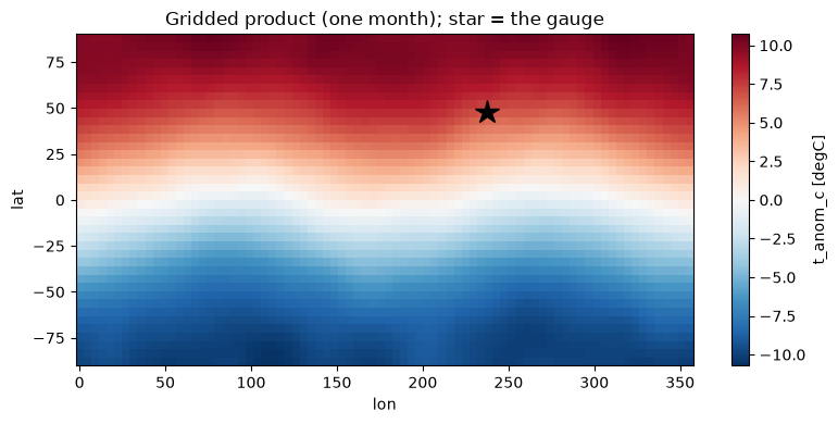
Space: .sel versus .interp
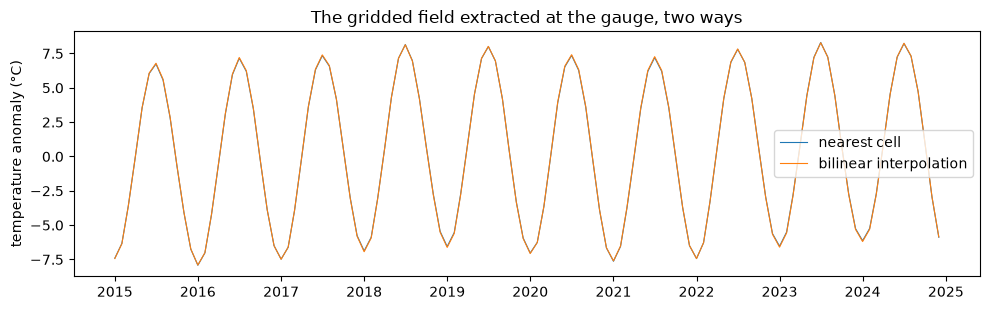
xarray gives both estimators in one line each: .sel(..., method="nearest") snaps to the closest cell center, .interp(...) interpolates bilinearly from the four surrounding cells. For a smooth field like temperature, bilinear is the better point estimate; for a categorical raster (land cover, geological unit), interpolation is meaningless — averaging “granite” and “basalt” produces nonsense — and nearest is the only correct choice. State which you used: on this coarse grid (4.5°) the two differ, and on real km-scale problems the difference can dominate.
t_nearest = temp_grid.sel(lat=gauge_lat, lon=gauge_lon, method="nearest")
t_bilinear = temp_grid.interp(lat=gauge_lat, lon=gauge_lon)

print(f"gauge at ({gauge_lat:.1f}N, {gauge_lon:.1f}E); "
      f"nearest cell center at ({float(t_nearest.lat):.1f}N, {float(t_nearest.lon):.1f}E)")
print(f"RMS difference nearest vs bilinear: "
      f"{float(np.sqrt(((t_nearest - t_bilinear) ** 2).mean())):.3f} degC")

fig, ax = plt.subplots(figsize=(10, 3.2))
ax.plot(grid_time, t_nearest, lw=0.8, label="nearest cell")
ax.plot(grid_time, t_bilinear, lw=0.8, label="bilinear interpolation")
ax.set_ylabel("temperature anomaly (°C)")
ax.legend()
ax.set_title("The gridded field extracted at the gauge, two ways")
plt.tight_layout()
gauge at (47.6N, 237.6E); nearest cell center at (47.4N, 238.5E)
RMS difference nearest vs bilinear: 0.037 degC
Time: a causal merge
The extracted series is monthly; the feature table is daily. The tempting move is to interpolate the temperature to daily resolution — but linear interpolation between month centers uses the next month’s value, which is future information: a forecasting feature built that way leaks, exactly in the sense of section 7. The causal join is pandas.merge_asof(..., direction="backward"): each day receives the most recent available monthly value and nothing from the future. That is the right default for predictive features; smooth interpolation is fine for retrospective analysis, and the choice belongs in the data card either way.
We merge the covariate into a copy of the feature table and rerun the flood classifier on the section-5 features with and without it, using the shipped chronological split and train-only preprocessing.
from sklearn.linear_model import LogisticRegression
from sklearn.metrics import average_precision_score
from sklearn.pipeline import make_pipeline
from sklearn.preprocessing import StandardScaler

# Station-side table of the extracted covariate
t_station = (t_bilinear.drop_vars(["lat", "lon"]).to_dataframe().reset_index()
             .rename(columns={"time": "date"}))

# Causal merge onto the daily feature table (both sorted by date)
feat_g = pd.merge_asof(feat.reset_index().sort_values("date"), t_station,
                       on="date", direction="backward").set_index("date")
print(feat_g[["q_lag1", "t_anom_c", "event", "split"]].head(3))

tr = feat_g["split"] == "train"
te = feat_g["split"] == "test"
base_cols = [c for c in feat_g.columns if c.startswith(("q_lag", "doy_"))]

for cols, label in [(base_cols, "discharge features only"),
                    (base_cols + ["t_anom_c"], "+ gridded temperature")]:
    pipe = make_pipeline(StandardScaler(),
                         LogisticRegression(max_iter=2000, class_weight="balanced"))
    pipe.fit(feat_g.loc[tr, cols], feat_g.loc[tr, "event"])
    ap = average_precision_score(feat_g.loc[te, "event"],
                                 pipe.predict_proba(feat_g.loc[te, cols])[:, 1])
    print(f"average precision, {label}: {ap:.3f}")
q_lag1 t_anom_c event split
date
2015-01-08 35.717825 -7.432165 0 train
2015-01-09 37.612688 -7.432165 0 train
2015-01-10 35.942248 -7.432165 0 train
average precision, discharge features only: 0.722
average precision, + gridded temperature: 0.710
The score barely moves — and that is the honest outcome: this synthetic temperature field has no causal connection to the injected floods, and a correctly joined covariate that carries no information about the target should not change the metric. The point of this section is the join, which is now leakage-safe, unit-labeled, and reproducible; on a real project the same six lines pull reanalysis precipitation onto a gauge, SST onto a buoy, or soil moisture onto a borehole, and there the covariate often carries the skill.
What the synthetic grid spared us, and a real one will not: reprojecting between coordinate reference systems (rioxarray/rasterio for anything in a projected CRS), the 0–360 vs ±180 longitude check we flagged above, the fact that a grid-cell value is an area average rather than a point measurement (a representativeness error that grows with terrain), and timestamp semantics (does “2015-01” stamp the start, middle, or end of the averaging interval?). Each of these is a data-card entry: the merged column’s provenance — source grid, extraction method, temporal join rule — is part of your dataset’s provenance now (checklist items 1 and 2).
7. Leakage by preprocessing
Checklist item 7, part one. Every statistic you compute from the data — a mean, a standard deviation, a PCA basis, an imputation value — is part of the model. If you compute it from the full dataset and then split, information from the test period has already flowed into the features the model trains on. This is leakage by preprocessing.
Here we standardize the features two ways:
- Wrong: fit
StandardScaleron all the data, then split and train. - Right: split first, fit the scaler on the training data only, and apply it (frozen) to the test data.
The floods in the test years shift the full-data mean and variance, so the wrong version quietly tells the model something about the test period. We score with average precision (area under the precision-recall curve), the appropriate metric for a rare positive class — accuracy would be ~97% for a model that never predicts a flood.
from sklearn.linear_model import LogisticRegression
from sklearn.metrics import average_precision_score
from sklearn.preprocessing import StandardScaler

train_mask = feat["split"] == "train"
test_mask = feat["split"] == "test"
X_train, y_train = X[train_mask], y[train_mask]
X_test, y_test = X[test_mask], y[test_mask]

# WRONG: scaler sees the test data
scaler_leaky = StandardScaler().fit(X)
clf = LogisticRegression(max_iter=2000, class_weight="balanced")
clf.fit(scaler_leaky.transform(X_train), y_train)
ap_leaky = average_precision_score(y_test, clf.predict_proba(scaler_leaky.transform(X_test))[:, 1])

# RIGHT: scaler sees only the training data
scaler_clean = StandardScaler().fit(X_train)
clf = LogisticRegression(max_iter=2000, class_weight="balanced")
clf.fit(scaler_clean.transform(X_train), y_train)
ap_clean = average_precision_score(y_test, clf.predict_proba(scaler_clean.transform(X_test))[:, 1])

print(f"average precision, scaler fit on ALL data (leaky): {ap_leaky:.3f}")
print(f"average precision, scaler fit on TRAIN only:       {ap_clean:.3f}")
print("\nScaler means for q_lag1 differ because the test years contain floods:")
print(f"  full-data mean: {scaler_leaky.mean_[0]:.3f}   train-only mean: {scaler_clean.mean_[0]:.3f}")
average precision, scaler fit on ALL data (leaky): 0.722
average precision, scaler fit on TRAIN only: 0.722
Scaler means for q_lag1 differ because the test years contain floods:
full-data mean: 26.002 train-only mean: 25.948
On this dataset the two scores are essentially identical: the series is long, roughly stationary, and a scaler carries only two numbers per feature, which a logistic regression can absorb into its weights. Do not take comfort in that. The gap grows when data are short, when the test period drifts away from the training period, or when the preprocessing is richer than a scaler — PCA bases, imputation models, feature selection, and normalization by global percentiles all leak far more than a mean and a standard deviation. The discipline costs nothing: split first, then fit every preprocessing step on the training split only. In sklearn, put the scaler and the model in a single Pipeline so cross-validation refits the preprocessing inside each fold automatically.
A leak that wrecks the metric: oversampling before the split
Here is a preprocessing leak with teeth, and one of the most common mistakes with rare events. To fight class imbalance, students often oversample the rare class — duplicate flood days until the classes are balanced — and then split randomly into train and test. The duplicated copies of the same flood day land on both sides of the split. The model is then tested on exact copies of its training samples.
from sklearn.ensemble import RandomForestClassifier
from sklearn.model_selection import train_test_split
from sklearn.utils import resample

Xa, ya = X.to_numpy(), y.to_numpy()

# WRONG: balance the classes first, split second
X_pos_up, y_pos_up = resample(Xa[ya == 1], ya[ya == 1],
                              n_samples=int((ya == 0).sum()), random_state=0)
X_bal = np.vstack([Xa[ya == 0], X_pos_up])
y_bal = np.concatenate([ya[ya == 0], y_pos_up])
X_tr, X_te, y_tr, y_te = train_test_split(X_bal, y_bal, test_size=0.3,
                                          random_state=0, stratify=y_bal)
rf = RandomForestClassifier(n_estimators=200, random_state=0).fit(X_tr, y_tr)
ap_wrong = average_precision_score(y_te, rf.predict_proba(X_te)[:, 1])

# RIGHT: split first, oversample the training set only
X_tr, X_te, y_tr, y_te = train_test_split(Xa, ya, test_size=0.3,
                                          random_state=0, stratify=ya)
X_pos_up, y_pos_up = resample(X_tr[y_tr == 1], y_tr[y_tr == 1],
                              n_samples=int((y_tr == 0).sum()), random_state=0)
rf = RandomForestClassifier(n_estimators=200, random_state=0).fit(
    np.vstack([X_tr[y_tr == 0], X_pos_up]),
    np.concatenate([y_tr[y_tr == 0], y_pos_up]))
ap_right = average_precision_score(y_te, rf.predict_proba(X_te)[:, 1])

print(f"average precision, oversample BEFORE split (leaky): {ap_wrong:.3f}")
print(f"average precision, oversample train only:           {ap_right:.3f}")
average precision, oversample BEFORE split (leaky): 1.000
average precision, oversample train only: 0.848
The leaky version reports a perfect or near-perfect score — pure fiction, produced entirely by duplicated samples straddling the split. Any preprocessing that creates, duplicates, selects, or transforms samples using knowledge of the whole dataset must happen inside the training split, never before it.
8. Splits for autocorrelated data
Checklist item 7, part two, and the biggest source of inflated scores in geoscience ML. Our features are seven-day windows of a smooth series: day and day have six of seven lag values in common. A random split scatters the days of a single flood across train and test. The model then “predicts” a test day by having memorized its near-duplicate neighbors in training. The score is real; the skill is not, and it will not transfer to a flood the model has never seen.
The fix is to split along the correlation structure:
TimeSeriesSplittrains on the past and tests on the future — the deployment scenario for forecasting.GroupKFoldkeeps groups intact: all days of one flood event stay on the same side of the split. We group flood days byevent_idand background days into monthly blocks.
One more deliberate choice: we switch from logistic regression to a random forest. A linear model has almost no capacity to memorize individual samples, so it hides the split problem. A random forest memorizes near-duplicates happily — and that capacity is exactly what a random split rewards. We run the identical pipeline (scaler + classifier, so preprocessing refits inside each fold) under the three cross-validation schemes.
from sklearn.ensemble import RandomForestClassifier
from sklearn.model_selection import GroupKFold, KFold, TimeSeriesSplit, cross_val_score
from sklearn.pipeline import make_pipeline

pipe = make_pipeline(StandardScaler(),
                     RandomForestClassifier(n_estimators=200, random_state=0,
                                            class_weight="balanced"))

# Groups: one group per flood event; background days grouped by 30-day block
day_index = np.arange(len(feat))
groups = np.where(feat["event_id"] >= 0,
                  feat["event_id"],
                  1000 + day_index // 30)

cv_schemes = {
    "KFold (random, shuffled)": (KFold(n_splits=5, shuffle=True, random_state=0), None),
    "TimeSeriesSplit": (TimeSeriesSplit(n_splits=5), None),
    "GroupKFold (by event)": (GroupKFold(n_splits=5), groups),
}

results = {}
for name, (cv, g) in cv_schemes.items():
    scores = cross_val_score(pipe, X, y, cv=cv, groups=g,
                             scoring="average_precision")
    results[name] = scores
    print(f"{name:28s} AP = {scores.mean():.3f} +/- {scores.std():.3f}")
KFold (random, shuffled) AP = 0.839 +/- 0.034
TimeSeriesSplit AP = 0.704 +/- 0.039
GroupKFold (by event) AP = 0.732 +/- 0.053
fig, ax = plt.subplots(figsize=(7, 3.5))
ax.boxplot([results[k] for k in cv_schemes], tick_labels=list(cv_schemes))
ax.set_ylabel("average precision")
ax.set_title("The same model, three ways of splitting the same data")
plt.tight_layout()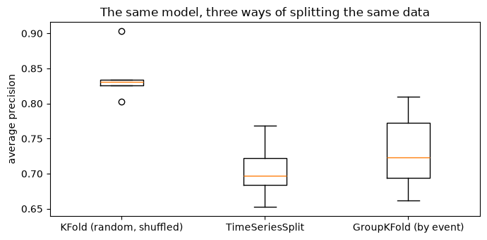
The random KFold reports the highest score by a wide margin, and it is the least trustworthy of the three: its test folds are full of samples that are near-copies of training samples, so the forest is graded on floods it has effectively already seen. TimeSeriesSplit and GroupKFold answer the question you actually care about — does the model detect floods it has never seen? — and they answer it less flatteringly. (TimeSeriesSplit also scores lowest in part because its early folds train on only a fraction of the data.)
Rules of thumb:
- Time series → split in time (
TimeSeriesSplit, or a chronological hold-out like our shippedsplitcolumn). - Event-based data (earthquakes, storms, floods) → split by event (
GroupKFoldon the event identifier). Never let windows from one event straddle the split. - Spatial data → split by region, not by pixel; nearby pixels are near-duplicates.
- When in doubt, ask: could a sample in the test set be trivially reconstructed from samples in the training set? If yes, the split is wrong.
This is why checklist item 6 says splits ship with the data: the dataset builder knows the correlation structure better than any downstream user, and a stored split makes every published score comparable.
9. Training, validation, and test sets
What is the role of a training and a test set
A training data set is the foundation of machine learning models. It provides the data used by the algorithm to learn patterns, relationships, and representations necessary for making predictions or decisions. The primary goal of the training data set is to enable the model to minimize the error or loss function by optimizing its parameters.
A test data set is used to evaluate the performance of the model on unseen data. Preparing it involves:
- Data Splitting: The test set is a subset of the data, separate from the training set, often 10-30% of the dataset — chosen with the correlation structure in mind, as above.
- Hold-Out Principle: Test data should never overlap with training or validation data, and it should be touched once, at the end. Every time you peek at test scores and change the model in response, the test set degrades into a validation set.
- Real-World Representativeness: The test data should reflect the scenarios where the model will be deployed, ensuring a robust performance evaluation.
Classic Machine Learning (CML) vs Deep Learning (DL)
CML: models are simpler, with fewer hyperparameters to tune (hyperparameters are the settings you choose before training — tree depth, learning rate — as opposed to the parameters the model learns from the data). A training set is used to fit the model, which is then evaluated on the test set. Cross-validation (as in section 8) assesses performance and reduces overfitting, often removing the need for a separate validation set.
DL: models are complex, often with millions of parameters, and need a validation set in addition to training and test sets. The validation set is used during training to tune hyperparameters (learning rate, number of layers) and to monitor overfitting (early stopping when validation loss stops improving).
A typical split for DL:
- Training set: 70-80% of the data.
- Validation set: 10-20% of the data.
- Test set: 10-20% of the data.
The validation set protects the test set: hyperparameter tuning consumes the validation set, so the test set remains genuinely unseen.
10. This checklist is graded
The AI-ready dataset you build for your project milestone will be evaluated against the checklist in section 1: provenance and license, a data card, tidy shapes and units, a missing-data policy, shipped benchmark splits, leakage controls, and a class/event inventory. See the chapter assignment and the final project description.
If you remember one sentence from this pillar: the split and the preprocessing are part of the dataset, not an afterthought of the model.