Introduction
In geosciences, much of the data we deal with — seismic waves, ocean tides, atmospheric pressure variations — comes in the form of time series. These signals often contain information at multiple frequencies, and a simple time-domain analysis may obscure important features of the data.
Spectrograms are useful tools for analyzing and visualizing the frequency content of time-series data. A spectrogram represents the spectral density of a signal as it changes over time. It is especially useful in geoscientific applications where signals are non-stationary, i.e., their frequency content changes over time. Examples include:
- Earthquake seismology: where both low and high-frequency signals are relevant at different stages of an event.
- Atmospheric science: where periodic patterns such as tides and waves have distinct frequency components.
- Remote sensing: where different processes, such as soil moisture fluctuations, can exhibit characteristic frequencies over time.
Why spectrograms matter
- Time-frequency analysis: Spectrograms show how the frequency content of a signal evolves over time, making them suitable for studying non-stationary data.
- Feature extraction: Spectrograms highlight transient events and long-duration patterns, useful for detecting and characterizing geophysical phenomena like earthquakes, landslides, or atmospheric waves.
- Multiscale analysis: Many natural processes operate at different time scales. Spectrograms let us visualize and extract features across these scales.
- Visualization: They offer a compact and interpretable visualization of complex time-series data.
In this section, we transform the data by projecting it onto a basis of functions. The two most used transforms are the Fourier and the wavelet transforms.
Warning. Filtering any data needs to be done carefully. Filtering artifacts can lead to complete misinterpretation. Common pitfalls:
- Not all filters preserve causality: some signals may appear before events and be misinterpreted as precursors.
- Filtering over data gaps brings high-frequency artifacts.
- Edge effects when filtering time series are difficult to mitigate.
The lecture covers several levels and methods for transforming data.
- Fourier Transforms: 1D [Level 1]
- Fourier Transforms: 2D [Level 3]
- Spectrograms [Level 2]
- Wavelet Transforms [Level 3]
# Import modules for seismic data and feature extraction

import os

import numpy as np
import matplotlib.pyplot as plt
import scipy
import scipy.signal as signal

# seismic python toolbox
import obspy
import obspy.clients.fdsn.client as fdsn
from obspy import UTCDateTime

os.makedirs('data', exist_ok=True)
We first download data: seismograms recorded in the Puget Sound for the M8.2 Chignik, Alaska earthquake of July 29, 2021. We query the FDSN data center with the IRIS client. Note that IRIS data services are now operated by EarthScope, but the client name IRIS still works.
The channel code HHZ denotes a high-gain broadband seismometer (H), sampled at 100 samples per second (H), vertical component (Z). This is a broadband channel: it records ground motion over a wide frequency band, not a single frequency.
We also download the station metadata (the instrument response) and remove the response with remove_response(output="VEL"). This converts the raw digitizer counts to ground velocity in m/s, so the amplitudes have physical units.
# Download seismic data
network = 'UW'
station = 'RATT'
channel = 'HHZ'  # broadband high-gain vertical channel, 100 samples per second
Tstart = UTCDateTime(2021, 7, 29, 6, 15)
Tend = Tstart + 7200
fdsn_client = fdsn.Client('IRIS')  # client to query the EarthScope (formerly IRIS) DMC server

# download the station metadata, including the instrument response
inv = fdsn_client.get_stations(network=network, station=station, channel=channel,
                               starttime=Tstart - 7200, endtime=Tend, level='response')

# call to download the specific data: earthquake waveforms
Z = fdsn_client.get_waveforms(network=network, station=station, location='--', channel=channel,
                              starttime=Tstart, endtime=Tend)
# basic pre-processing: merge if there are gaps, detrend, taper,
# then remove the instrument response to convert digitizer counts to ground velocity (m/s).
Z.merge(); Z.detrend(type='linear'); Z[0].taper(max_percentage=0.05)
Z.remove_response(inventory=inv, output="VEL")

# call to download the specific data: noise waveforms (the two hours before the earthquake)
N = fdsn_client.get_waveforms(network=network, station=station, location='--', channel=channel,
                              starttime=Tstart - 7200, endtime=Tstart)
N.merge(); N.detrend(type='linear'); N[0].taper(max_percentage=0.05)
N.remove_response(inventory=inv, output="VEL")
/home/runner/work/mlgeo-book/mlgeo-book/.pixi/envs/default/lib/python3.12/site-packages/obspy/clients/fdsn/client.py:251: ObsPyDeprecationWarning: IRIS is now EarthScope, please consider changing the FDSN client short URL to 'EARTHSCOPE'.
warnings.warn(msg, ObsPyDeprecationWarning)
1 Trace(s) in Stream:
UW.RATT..HHZ | 2021-07-29T04:15:00.000000Z - 2021-07-29T06:14:59.990000Z | 100.0 Hz, 720000 samples
plt.plot(Z[0].data); plt.plot(N[0].data); plt.grid(True)
plt.ylabel('Velocity (m/s)'); plt.xlabel('Sample index')
plt.legend(['Earthquake', 'Noise'])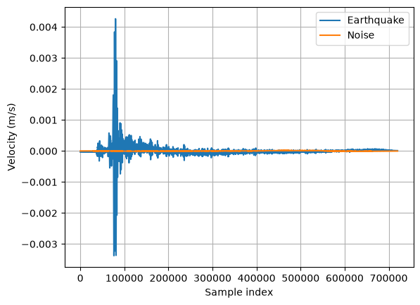
1. Fourier Transforms [Level 1]
We use the scipy.fft module to transform the two time series (earthquake and noise). The older scipy.fftpack module is legacy and should no longer be used.
The Fourier transform is a decomposition of the time series onto an orthonormal basis of cosine and sine functions. The Fourier transform of a time series (similarly if the variable is space ) is:
is the complex Fourier value at frequency . The Fourier transform determines what frequencies dominate the time series.
1.1 Nyquist
The Fourier transform we use in this class takes a discrete time series of real numbers. If the time series spans seconds with regularly spaced samples, the sampling interval is . The highest frequency that can be resolved in a discrete time series, called the Nyquist frequency, is limited by :
Effectively, one cannot constrain signals that vary faster than two time samples. Here s, so Hz.
1.2 Uncertainties
- The discrete Fourier Transform yields an approximation of the FT. The shorter the time series, the less accurate the FT. This means that the FT on short time windows is less accurate.
- The FT assumes (and requires) periodicity of the series, meaning that the finite/trimmed time series would repeat in time. To enforce this, we taper the time series so that the first and last points are equal (to zero).
from scipy.fft import fft, ifft, fftfreq, next_fast_len

npts = Z[0].stats.npts

## FFT the signals
# pad up to a fast FFT length to speed up the FFT
Nfft = next_fast_len(int(Z[0].data.shape[0]))  # this will be an even number

freqVec = fftfreq(Nfft, d=Z[0].stats.delta)[:Nfft//2]

Z.taper(max_percentage=0.05)

Zhat = fft(Z[0].data, n=Nfft)
Please see the Obspy documentation to find out about the taper function. Plot the amplitude and phase spectra.
fig, ax = plt.subplots(2, 1, figsize=(11, 8))
ax[0].plot(freqVec, np.abs(Zhat[:Nfft//2])/Nfft)
ax[0].grid(True)
ax[0].set_xscale('log'); ax[0].set_yscale('log')
ax[0].set_xlabel('Frequency (Hz)'); ax[0].set_ylabel('Amplitude (m/s)')
ax[0].set_title('Amplitude spectrum, earthquake')

ax[1].hist(np.angle(Zhat[:Nfft//2]))
ax[1].grid(True)
ax[1].set_xlabel('Phase (radians)'); ax[1].set_ylabel('Count')
ax[1].set_title('Distribution of the phase spectrum')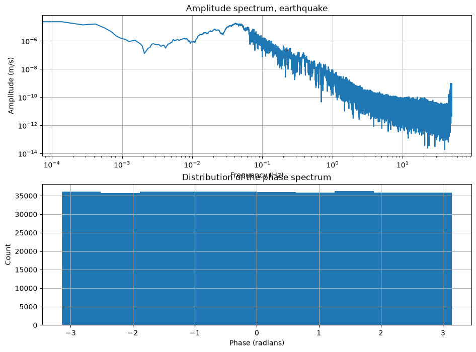
You will note above that the phase values are randomly distributed between and π. We can check it by showing the distribution of the phase and amplitude spectra.
# your turn. Plot the histogram of the amplitude spectrum
plt.hist(np.log10(np.abs(Zhat[:Nfft//2])/Nfft), 100); plt.grid(True)
plt.xlabel('log10 amplitude'); plt.ylabel('Count')
plt.show()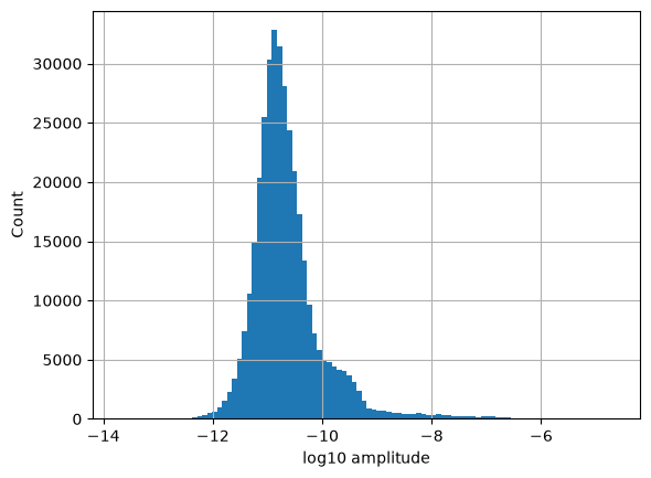
We can also analyze the spectral characteristics of the noise time series. Below:
- compute the Fourier transform
- plot the phase and amplitude spectra
- plot the distribution of the phase and amplitude values
# compute Fourier transform of the noise time series

npts1 = N[0].stats.npts
## FFT the signals
# pad up to a fast FFT length to speed up the FFT
Nfft1 = next_fast_len(int(N[0].data.shape[0]))  # this will be an even number
freqVec1 = fftfreq(Nfft1, d=N[0].stats.delta)[:Nfft1//2]

# taper the data to enforce periodicity
N.taper(max_percentage=0.05)

# Fourier transform
Nhat = fft(N[0].data, n=Nfft1)
# plot the phase and amplitude spectra
fig, ax = plt.subplots(2, 1, figsize=(11, 8))
ax[0].plot(freqVec1, np.abs(Nhat[:Nfft1//2])/Nfft1)
ax[0].grid(True)
ax[0].set_xscale('log'); ax[0].set_yscale('log')
ax[0].set_xlabel('Frequency (Hz)'); ax[0].set_ylabel('Amplitude (m/s)')
ax[0].set_title('Amplitude spectrum, noise')
ax[1].hist(np.angle(Nhat[:Nfft1//2]))
ax[1].grid(True)
ax[1].set_xlabel('Phase (radians)'); ax[1].set_ylabel('Count')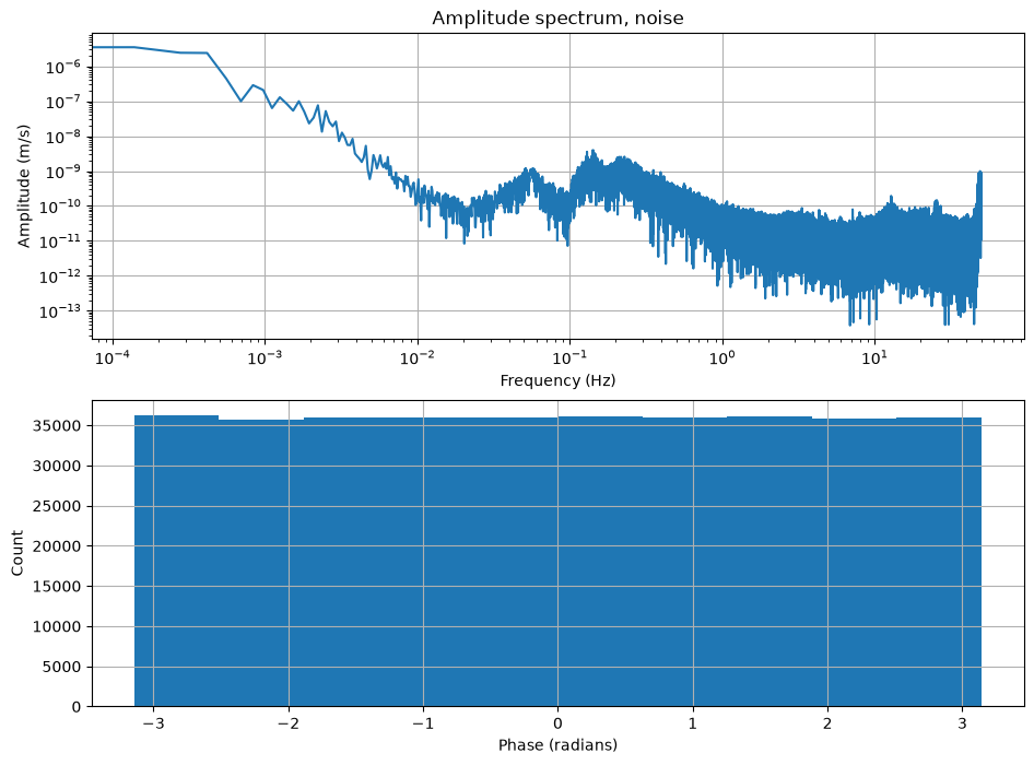
# Overlay the spectrum of the earthquake and the spectrum of the noise

fig, ax = plt.subplots(1, 1, figsize=(11, 8))
ax.plot(freqVec, np.abs(Zhat[:Nfft//2])/Nfft)
ax.plot(freqVec1, np.abs(Nhat[:Nfft1//2])/Nfft1)
ax.grid(True)
ax.set_xscale('log'); ax.set_yscale('log')
ax.set_xlabel('Frequency (Hz)'); ax.set_ylabel('Amplitude (m/s)')
ax.legend(['Earthquake', 'Noise'])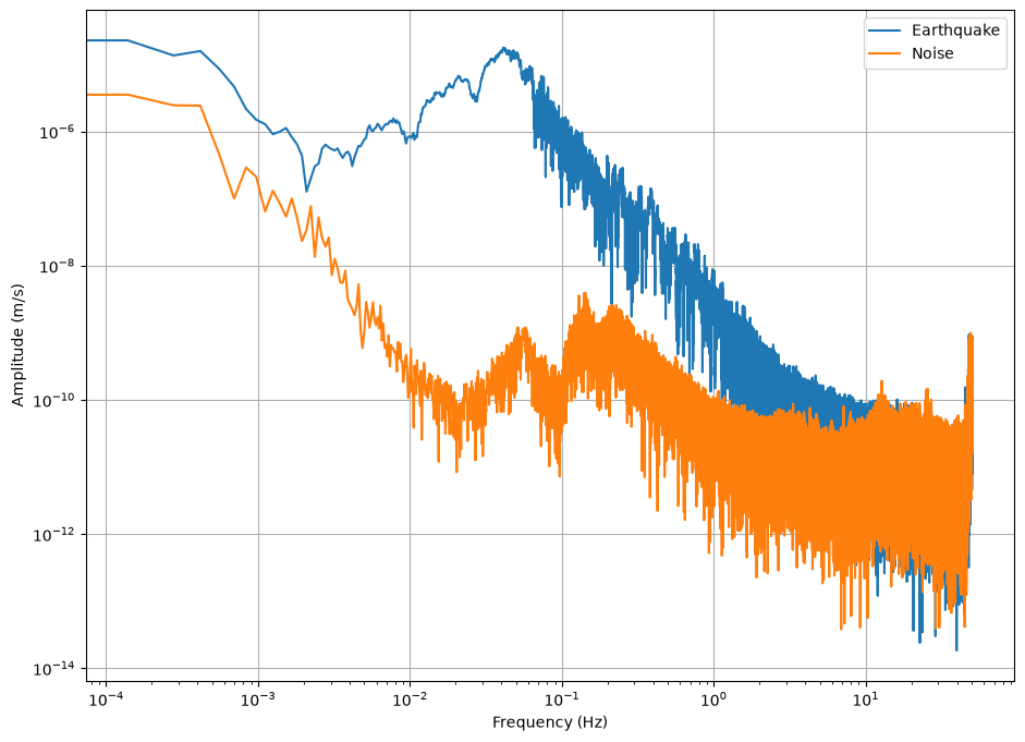
Overlay their PDFs.
# your turn. Plot the histograms of the amplitude spectra
plt.hist(np.log10(np.abs(Zhat[:Nfft//2])/Nfft), 100)
plt.hist(np.log10(np.abs(Nhat[:Nfft1//2])/Nfft1), 100)
plt.grid(True)
plt.xlabel('log10 amplitude'); plt.ylabel('Count')
plt.legend(['Earthquake', 'Noise'])
plt.show()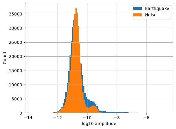
You notice that their statistical differences are in the tails of the distributions. Therefore, statistical metrics such as mean or variance may not be discriminatory, but kurtosis might.
# print short float values
print(f"Skewness of earthquake {scipy.stats.skew(np.log10(np.abs(Zhat[:Nfft//2])))} and noise {scipy.stats.skew(np.log10(np.abs(Nhat[:Nfft1//2])))}")

print(f"Kurtosis of earthquake {scipy.stats.kurtosis(np.log10(np.abs(Zhat[:Nfft//2])))} and noise {scipy.stats.kurtosis(np.log10(np.abs(Nhat[:Nfft1//2])))}")

print(f"Mean of earthquake {np.mean(np.log10(np.abs(Zhat[:Nfft//2])))} and noise {np.mean(np.log10(np.abs(Nhat[:Nfft1//2])))}")

print(f"standard deviation of earthquake {np.std(np.log10(np.abs(Zhat[:Nfft//2])))} and noise {np.std(np.log10(np.abs(Nhat[:Nfft1//2])))}")
Skewness of earthquake 2.4536951625724006 and noise 0.7840246929880924
Kurtosis of earthquake 11.193100408193848 and noise 2.7513010817144057
Mean of earthquake -4.77249112779935 and noise -4.872561055684667
standard deviation of earthquake 0.7077083875874777 and noise 0.43451042923912164
2. 2D Fourier Transforms [Level 3]
The 2D Fourier transform is applied to a 2D matrix. It first applies a 1D Fourier transform to every row of the matrix, then applies a 1D Fourier transform to every column of the intermediate matrix.
2D Fourier transforms give the Fourier coefficients that dominate an image. This can be used for filtering the data. Another application is to compress the data by keeping a few coefficients instead of storing the whole image.
We will practice on a synthetic topography-like field. Real topography has a “red” wavenumber spectrum: most of the power sits at long wavelengths (mountain ranges), with progressively less power at short wavelengths (small-scale roughness). The spectral amplitude decays roughly as a power law of the wavenumber , . We can build such a fractal terrain directly in the Fourier domain: draw random phases, scale the amplitudes by , and inverse transform.
from scipy.fft import fft2, ifft2, fftshift
from scipy.fft import fftfreq as fftfreq2d

# build a synthetic fractal terrain with a power-law (red) wavenumber spectrum
rng = np.random.default_rng(42)

nx, ny = 512, 512      # grid size
dx = 1.0               # grid spacing in km
beta = 2.0             # spectral decay exponent: amplitude ~ k^-beta

# wavenumber grids (cycles per km)
kx = fftfreq2d(nx, d=dx)
ky = fftfreq2d(ny, d=dx)
KX, KY = np.meshgrid(kx, ky, indexing='ij')
K = np.sqrt(KX**2 + KY**2)
K[0, 0] = np.inf  # avoid division by zero at the zero wavenumber (mean)

# random phases on a white-noise field, amplitudes scaled by k^-beta
white = rng.standard_normal((nx, ny))
shaped = fft2(white) * K**(-beta)
elevation = np.real(ifft2(shaped))

# rescale to a plausible elevation range in meters
elevation = 2000 * (elevation - elevation.min()) / (elevation.max() - elevation.min())

# spatial coordinate vectors in km
xkm = np.arange(nx) * dx
ykm = np.arange(ny) * dx

plt.figure(figsize=(7, 6))
plt.contourf(xkm, ykm, elevation.T, 30, cmap='terrain')
plt.colorbar(label='Elevation (m)')
plt.xlabel('x (km)'); plt.ylabel('y (km)')
plt.title('Synthetic fractal terrain')
plt.axis('scaled')
plt.show()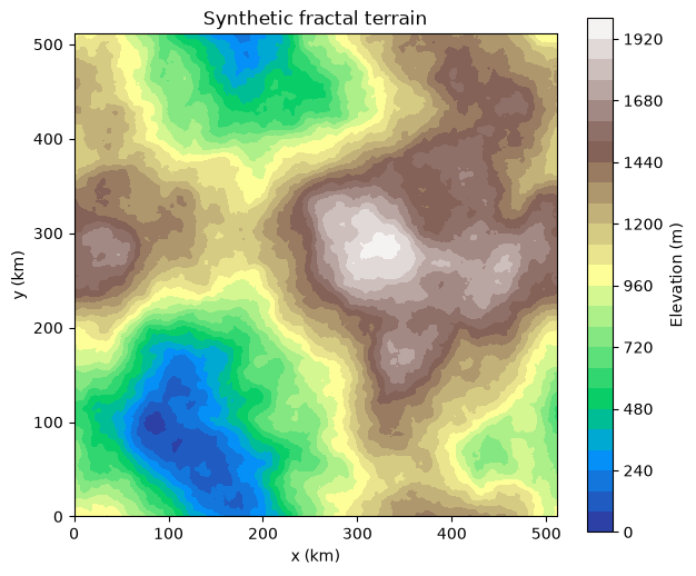
Consider elevation as a 2D data set. We can perform a 2D transform, which gives a spectrum in the spatial dimensions. The axes of the transformed image are wavenumbers (cycles per km). We use fftshift to place the zero wavenumber at the center of the image.
Zel = fft2(elevation)

kmax = 1 / (2 * dx)  # Nyquist wavenumber in cycles per km

plt.figure(figsize=(7, 6))
plt.imshow(fftshift(np.log10(np.abs(Zel) / Zel.size)), cmap='RdYlBu',
           extent=[-kmax, kmax, -kmax, kmax])
plt.colorbar(label='log10 amplitude')
plt.xlabel('$k_x$ (km$^{-1}$)'); plt.ylabel('$k_y$ (km$^{-1}$)')
plt.title('2D FT of elevation')
plt.show()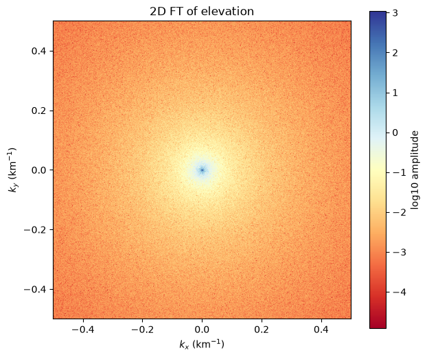
The energy is concentrated near the center of the plot (low wavenumbers, long wavelengths), as designed. Now we will compress the image by keeping only the largest Fourier coefficients.
# Sort the Fourier coefficient amplitudes
Zsort = np.sort(np.abs(Zel).reshape(-1))
print(len(Zsort))
print(Zsort.shape)
262144
(262144,)
fig, ax = plt.subplots(1, 3, figsize=(12, 4), sharey=True)
for i, keep in enumerate((0.1, 0.05, 0.01)):
    thresh = Zsort[int(np.floor((1 - keep) * len(Zsort)))]
    ind = np.abs(Zel) > thresh
    Atlow = Zel * ind  # zero out the small coefficients
    Alow = np.real(ifft2(Atlow))
    ax[i].contourf(xkm, ykm, Alow.T, 30, cmap='terrain')
    ax[i].set_title(f'keep {keep*100:.0f}% of coefficients')
    ax[i].axis('scaled')
    ax[i].set_xlabel('x (km)')
ax[0].set_ylabel('y (km)')
plt.show()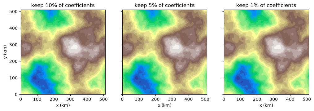
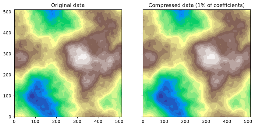
Now we compare the original 2D data set with the Fourier-compressed data. Keeping 1% of the coefficients is a compression ratio of 100:1, and the reconstruction still captures the large-scale structure of the terrain. The price is the loss of the small-scale roughness, which lives in the discarded high-wavenumber coefficients.
keep = 0.01
thresh = Zsort[int(np.floor((1 - keep) * len(Zsort)))]
ind = np.abs(Zel) > thresh
Atlow = Zel * ind  # zero out the small coefficients
print("We are keeping %.2f%% of the Fourier coefficients, a compression ratio of %d:1" % (keep*100, int(1/keep)))
Alow = np.real(ifft2(Atlow))

fig, ax = plt.subplots(1, 2, figsize=(10, 5), sharex=True, sharey=True)
ax[0].contourf(xkm, ykm, elevation.T, 30, cmap='terrain'); ax[0].set_title('Original data')
ax[0].axis('scaled')
ax[1].contourf(xkm, ykm, Alow.T, 30, cmap='terrain'); ax[1].set_title('Compressed data (1% of coefficients)')
ax[1].axis('scaled')

# quantify the reconstruction error
rel_err = np.linalg.norm(elevation - Alow) / np.linalg.norm(elevation)
print(f"Relative reconstruction error: {rel_err:.3f}")
We are keeping 1.00% of the Fourier coefficients, a compression ratio of 100:1
Relative reconstruction error: 0.006
3. Spectrograms [Level 2]
In time-dependent and multi-scale problems, it may be interesting to extract data features from the short time Fourier transform (STFT).
The STFT is a Fourier Transform applied to short (overlapping) windows to resolve the frequencies over different times in the series.
from scipy.signal import stft

fs = Z[0].stats.sampling_rate
nperseg = 1000
z = np.asarray(Z[0].data)
f, t, Zxx = stft(z, fs=fs, nperseg=nperseg, noverlap=200)
fig, ax = plt.subplots(2, 1, figsize=(11, 8), sharex=True)
logZ = np.log10(np.abs(Zxx) + 1e-20)
ax[0].pcolormesh(t/3600, f, logZ, vmin=np.percentile(logZ, 50), vmax=np.percentile(logZ, 99.9), shading='gouraud')
ax[0].set_title('STFT Magnitude, earthquake')
ax[0].set_ylabel('Frequency [Hz]')
ax[0].set_yscale('log'); ax[0].set_ylim(0.1, 40)

n = np.asarray(N[0].data)
fn, tn, Nxx = stft(n, fs=fs, nperseg=nperseg, noverlap=200)
logN = np.log10(np.abs(Nxx) + 1e-20)
ax[1].pcolormesh(tn/3600, fn, logN, vmin=np.percentile(logN, 50), vmax=np.percentile(logN, 99.9), shading='gouraud')
ax[1].set_title('STFT Magnitude, noise')
ax[1].set_ylabel('Frequency [Hz]')
ax[1].set_xlabel('Time [Hours]'); ax[1].set_yscale('log'); ax[1].set_ylim(0.1, 40)
(0.1, 40)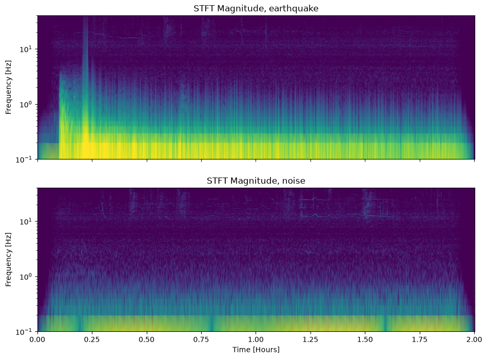
The spectrogram Zxx is a transform of the original data. It is common to use spectrograms as input to neural networks as 2D arrays.
Zxx.shape(501, 902)4. Continuous Wavelet Transform [Level 3]
Introduction
The Continuous Wavelet Transform (CWT) is an important tool in geoscientific data analysis, particularly for time-frequency analysis of non-stationary signals. Like the spectrogram, the CWT provides insight into how the frequency content of a signal varies over time. However, the CWT offers better resolution at different frequencies, making it more suitable for analyzing signals with transient or localized frequency changes.
The wavelet transform breaks a signal down into scaled and shifted versions of a small, oscillating function known as the wavelet. This makes the CWT well-suited for geoscientific applications, where many phenomena, such as earthquakes, volcanic eruptions, and weather patterns, can manifest at different scales and frequencies.
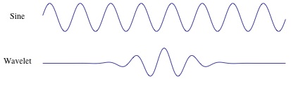
Figure: Fourier and wavelet basis functions. Image from this article.
There exist many canonical wavelet families. The difference between families is typically their shape, compactness, and smoothness. Typically, one chooses one family for the specific time series. Wavelets have finite energy and zero mean.
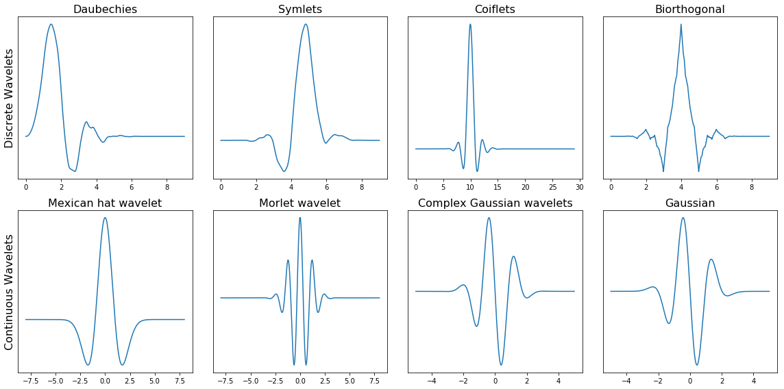
Figure: Families of wavelet basis functions. Image from this article
The wavelet transform is:
where is the mother wavelet scaled by a factor of and translated/shifted by . In the continuous transform, and take continuous values. The Discrete Wavelet Transform is the wavelet transform performed on a finite number of scales and shifts.
The time-scale representation of a time series is a scaleogram. Scales can be converted to pseudo-frequencies: if is the central frequency of the wavelet, the scale is , and the sampling interval is , then the pseudo-frequency is .
Why Continuous Wavelet Transforms are Important
- Multiresolution analysis: The CWT captures both low-frequency, long-duration trends and high-frequency, short-duration features. This is particularly valuable in geosciences, where processes occur on different temporal and spatial scales.
- Non-stationary data: Many geoscientific signals are non-stationary, meaning their statistical properties change over time. The CWT reveals these time-varying frequency components.
- Local feature detection: CWT is well suited for identifying localized events, such as seismic waves, landslides, or atmospheric disturbances, by analyzing how the signal changes in both time and frequency.
- Better time-frequency resolution: The wavelet transform provides more precise time and frequency localization than methods like the Fourier transform or spectrogram, especially for short-lived events.
Use in Seismology
In seismic data, different types of seismic waves (P-waves, S-waves, and surface waves) occur at different frequencies and durations. By applying CWT, seismologists can detect these different wave phases and their precise arrival times, which matter for earthquake characterization.
Python Example: Continuous Wavelet Transform of Seismic Data
We use the PyWavelets (pywt) package. The older scipy.signal.cwt and scipy.signal.morlet2 functions were removed from SciPy, so pywt is now the standard tool. We choose the complex Morlet wavelet 'cmor1.5-1.0' (bandwidth 1.5, center frequency 1.0), a common choice for seismic data because its complex form gives both amplitude and phase.
pywt.cwt works in scales. We pick the frequencies we want to resolve (0.1 to 40 Hz, log-spaced), then convert them to scales with the relation , which is what pywt.frequency2scale computes. To keep the computation light, we apply the CWT to the first 20 minutes of the earthquake record, which contains the P, S, and surface waves.
import pywt

fs = Z[0].stats.sampling_rate
dt = 1 / fs

# analyze the first 20 minutes of the earthquake record
nsel = int(1200 * fs)
zsel = z[:nsel]
tsel = np.arange(nsel) / fs

# choose the frequencies to resolve, then convert them to scales
wavelet = 'cmor1.5-1.0'
freqs_target = np.logspace(np.log10(0.1), np.log10(40), 100)
scales = pywt.frequency2scale(wavelet, freqs_target * dt)  # scales for the target frequencies

# compute the CWT; frequencies returned in Hz thanks to sampling_period
coefficients, frequencies = pywt.cwt(zsel, scales, wavelet, sampling_period=dt, method='fft')
print(coefficients.shape, frequencies.min(), frequencies.max())
(100, 120000) 0.1 39.99999999999999
# plot the scalogram with a frequency axis in Hz
logC = np.log10(np.abs(coefficients) + 1e-20)
plt.figure(figsize=(11, 5))
plt.pcolormesh(tsel, frequencies, logC, cmap='viridis',
               vmin=np.percentile(logC, 50), vmax=np.percentile(logC, 99.9), shading='auto')
plt.yscale('log')
plt.ylim(frequencies.min(), frequencies.max())
plt.colorbar(label='log10 |CWT coefficient|')
plt.xlabel('Time (s)')
plt.ylabel('Frequency (Hz)')
plt.title('Scalogram of the Chignik earthquake at UW.RATT (cmor1.5-1.0)')
plt.show()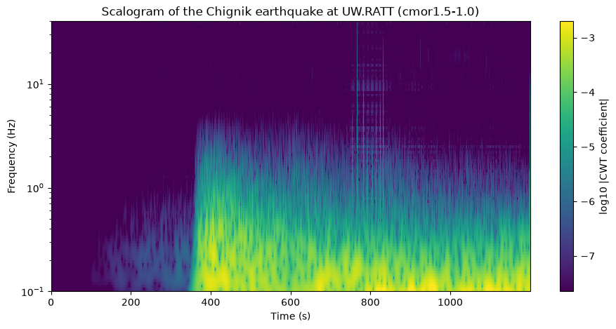
The scalogram shows the P wave arriving first with high-frequency energy, followed by the S wave and long-period surface waves below 0.1-0.5 Hz. Compare this with the STFT spectrogram above: the wavelet transform resolves the low-frequency surface waves better because its time window adapts to each frequency.
Advantages of CWT in Geosciences:
- Time-localized event detection: CWT identifies short-lived geophysical events, such as the arrival of seismic waves during an earthquake.
- Multiscale phenomena: Natural processes like tectonic activity and oceanic tides operate over a broad range of temporal and spatial scales. CWT can analyze signals from these processes by using a wide range of scales.
- Edge detection: The wavelet transform is particularly good at detecting changes or discontinuities in signals, such as the sharp onset of seismic waves or the boundaries of different geophysical layers.
Use Cases in Geoscience:
- Earthquake early warning: By applying CWT, geoscientists can more accurately detect the first arrival of seismic waves, which matters for early warning systems.
- Landslide detection: The CWT helps in identifying high-frequency signals indicative of landslides, as these events are often characterized by short bursts of energy.
- Volcanic tremors: CWT can be used to analyze volcanic tremor signals, which are often complex and exhibit both short and long-duration features.
Conclusion
The Continuous Wavelet Transform (CWT) is a useful tool for time-frequency analysis in geosciences. Its ability to resolve signals across different scales and frequencies makes it well suited for studying non-stationary processes. Python libraries like pywt, obspy, and matplotlib let geoscientists apply the CWT to their data and extract insight into complex geophysical phenomena.
Time-frequency transforms take computational time in a workflow. Let’s compare the cost of the CWT and the STFT on the same 20-minute segment.
import time

tic = time.perf_counter()
pywt.cwt(zsel, scales, wavelet, sampling_period=dt, method='fft')
toc = time.perf_counter()
print(f"CWT (100 scales, 20 min of data): {toc - tic:.2f} s")

tic = time.perf_counter()
stft(zsel, fs=fs, nperseg=nperseg, noverlap=200)
toc = time.perf_counter()
print(f"STFT (same data): {toc - tic:.3f} s")
CWT (100 scales, 20 min of data): 0.64 s
STFT (same data): 0.003 s
The STFT is much cheaper than the CWT. From these transforms, we can extract similar statistical features.