In this tutorial, we will manipulate the data structure from and to several data formats: JSON, CSV, Parquet, GeoTIFF, GeoJSON, netCDF/HDF5, and Zarr. At the end, we compare the on-disk size of the same data across formats.
All files created or downloaded in this notebook go into a local data/ folder.
import os

os.makedirs('data', exist_ok=True)
JSON (JavaScript Object Notation)
JSON is a lightweight, human-readable data format used in web applications and APIs for data exchange. JSON is used to store metadata, configuration files, and small datasets, particularly when working with web-based applications or interacting with APIs (e.g., querying weather data or geospatial information from an API). Here is a simple example:
{
    "location": "Yellowstone",
    "coordinates": {
        "latitude": 44.423691,
        "longitude": -110.588516
    },
    "elevation_m": 2399,
    "temperature_c": 22.5
}
The character encoding is UTF-8. The data types in JSON files may be numbers, string, boolean, array, object (collection of name-value pairs), or null. More information on JSON from the EarthDataScience course.
In Python, you create a JSON file with the json library:
import json

data = {
    "location": "Yellowstone",
    "coordinates": {"latitude": 44.423691, "longitude": -110.588516},
    "elevation_m": 2399,
    "temperature_c": 22.5
}

with open('data/data.json', 'w') as outfile:
    json.dump(data, outfile)
Tabular Data Formats
Tabular data are common in geosciences. The CSV format is a convenient, human-readable format for small data sets that stores data in rows. The Parquet format is machine-readable, columnar, and compressed, built for large data sets.
CSV (Comma-Separated Values):
CSV is a simple, widely used format for tabular data, often used in geoscience for sharing and storing smaller datasets (e.g., soil samples, environmental readings).
It stores data as plain text, making it easy to read but inefficient for large datasets. It is most often read using pandas.
import pandas as pd

# Build a small table and write it to a CSV file
df = pd.DataFrame({
    'station': ['RAIN', 'HELN', 'BAKR'],
    'temperature_c': [12.5, 10.1, 8.3],
    'precipitation_mm': [3.0, 1.2, 0.0],
})
df.to_csv('data/output.csv', index=False)

# Read it back
df = pd.read_csv('data/output.csv')
dfParquet:
Parquet is a binary, columnar storage format optimized for efficiency, particularly for large datasets. It is widely used in big data environments (e.g., storing satellite imagery or climate model outputs).
# Writing the same table to a Parquet file
df.to_parquet('data/output.parquet', index=False)

# Reading the Parquet file
df_read = pd.read_parquet('data/output.parquet')
print(df_read)
station temperature_c precipitation_mm
0 RAIN 12.5 3.0
1 HELN 10.1 1.2
2 BAKR 8.3 0.0
Geospatial Data
The main formats for geospatial data in this lesson are:
- GeoTIFF: a metadata standard that embeds georeferencing information in a TIFF (Tagged Image File Format) file. Cloud-Optimized GeoTIFF (COG) is a variant organized for remote access.
- GeoJSON: a format for encoding a variety of geographic data structures (points, lines, polygons) in JSON.
import folium
import geopandas as gpd
import h5py
import matplotlib.pyplot as plt
import netCDF4 as nc
import numpy as np
import pooch
import rasterio
import xarray as xr

from folium.plugins import MarkerCluster
from rasterio.plot import show
1. Raster data
1.1 rasterio to read GeoTIFF
Raster data is any pixelated (or gridded) data where each pixel is associated with a specific geographical location. The value of a pixel can be continuous (e.g., elevation) or categorical (e.g., land use).
The python package rasterio (documentation) reads formats such as GeoTIFF.
See additional introductory materials from EarthDataScience and tutorials from the GeoHackweek.
We will download a shaded-relief topography raster from Natural Earth. The file name is HYP_50M_SR and it comes as a zipped file. We use pooch to download it into data/ and unzip it in one step.
files = pooch.retrieve(
    url="https://naciscdn.org/naturalearth/50m/raster/HYP_50M_SR.zip",
    known_hash="sha256:de6faaee29c8707764852a36c0973aea184e8ec94b6eebf21d061c923c8025de",
    fname="HYP_50M_SR.zip",
    path="./data",
    processor=pooch.Unzip(extract_dir="HYP_50M_SR"),
)
tif_file = [f for f in files if f.endswith(".tif")][0]
print(tif_file)
Downloading data from 'https://naciscdn.org/naturalearth/50m/raster/HYP_50M_SR.zip' to file '/home/runner/work/mlgeo-book/mlgeo-book/book/Chapter2-DataManipulation/data/HYP_50M_SR.zip'.
Unzipping contents of '/home/runner/work/mlgeo-book/mlgeo-book/book/Chapter2-DataManipulation/data/HYP_50M_SR.zip' to '/home/runner/work/mlgeo-book/mlgeo-book/book/Chapter2-DataManipulation/data/HYP_50M_SR'
/home/runner/work/mlgeo-book/mlgeo-book/book/Chapter2-DataManipulation/data/HYP_50M_SR/HYP_50M_SR.tif
Now let’s open the GeoTIFF with rasterio.
elevation = rasterio.open(tif_file)A rasterio dataset is not a netCDF file: it has no .variables. Instead, it stores one or more bands. The basic attributes are .count (number of bands), .width and .height (raster dimensions), and .crs (coordinate reference system).
print("number of bands:", elevation.count)
print("width :", elevation.width)
print("height:", elevation.height)
print("crs   :", elevation.crs)
number of bands: 3
width : 10800
height: 5400
crs : EPSG:4326
elevation.indexes(1, 2, 3)Can you guess how to get the data types of the bands?
# type below
elevation.dtypes
('uint8', 'uint8', 'uint8')And the boundaries of the dataset:
elevation.boundsBoundingBox(left=-179.99999999999997, bottom=-89.99999999998201, right=179.99999999996405, top=90.0)print(elevation.transform * (0, 0)) # North West corner
print(elevation.transform * (elevation.width, elevation.height)) # South East corner(-179.99999999999997, 90.0)
(179.99999999996405, -89.99999999998201)
How to interpret the data: there are three bands, one for each of the colors red, green, and blue:
print(elevation.colorinterp[0])
print(elevation.colorinterp[1])
print(elevation.colorinterp[2])
3
4
5
print(np.min(elevation.read(1)), np.max(elevation.read(1)))
print(np.min(elevation.read(2)), np.max(elevation.read(2)))
print(np.min(elevation.read(3)), np.max(elevation.read(3)))
59 255
79 255
75 255
elevation.read(1) returns the first band as a 2D numpy array. Let us plot it alone, then all three bands as a color image.
band1 = elevation.read(1)
plt.imshow(band1, cmap='gray')
plt.colorbar(shrink=0.5, label='red band value')
plt.title('HYP_50M_SR, band 1')
plt.show()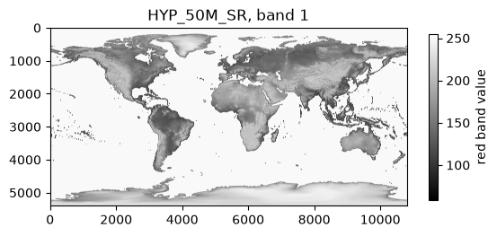
image = elevation.read()
show(image)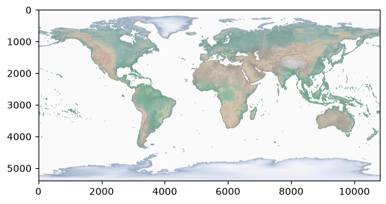
<Axes: >1.2 Geopandas to read GeoJSON
GeoJSON is a special case of JSON that stores geographic features (points, lines, polygons) with their attributes. Instead of downloading one, we will build a small GeoJSON from scratch: a FeatureCollection of four Cascade volcanoes. This shows the structure of the format explicitly.
volcanoes_geojson = {
    "type": "FeatureCollection",
    "features": [
        {
            "type": "Feature",
            "properties": {"name": "Mt Rainier", "elevation_m": 4392},
            "geometry": {"type": "Point", "coordinates": [-121.7603, 46.8523]},
        },
        {
            "type": "Feature",
            "properties": {"name": "Mt St Helens", "elevation_m": 2549},
            "geometry": {"type": "Point", "coordinates": [-122.1944, 46.1912]},
        },
        {
            "type": "Feature",
            "properties": {"name": "Mt Baker", "elevation_m": 3286},
            "geometry": {"type": "Point", "coordinates": [-121.8144, 48.7768]},
        },
        {
            "type": "Feature",
            "properties": {"name": "Glacier Peak", "elevation_m": 3213},
            "geometry": {"type": "Point", "coordinates": [-121.1132, 48.1125]},
        },
    ],
}

with open('data/cascade_volcanoes.geojson', 'w') as f:
    json.dump(volcanoes_geojson, f, indent=2)
Note the structure: each Feature has a geometry (here a Point with longitude first, then latitude) and a properties dictionary for the attributes. Now read the file back with geopandas:
volcanoes = gpd.read_file('data/cascade_volcanoes.geojson')
volcanoesGeopandas parsed the geometry column and set the coordinate reference system to WGS84 (EPSG:4326), the GeoJSON default:
volcanoes.crs<Geographic 2D CRS: EPSG:4326>
Name: WGS 84
Axis Info [ellipsoidal]:
- Lat[north]: Geodetic latitude (degree)
- Lon[east]: Geodetic longitude (degree)
Area of Use:
- name: World.
- bounds: (-180.0, -90.0, 180.0, 90.0)
Datum: World Geodetic System 1984 ensemble
- Ellipsoid: WGS 84
- Prime Meridian: GreenwichLet us plot the data on an interactive map. Folium is a nice Python package for visualization. The Geohackweek tutorial on Folium is also informative.
m = folium.Map(location=[47.5, -121.8], zoom_start=7)
marker_cluster = MarkerCluster().add_to(m)
for _, row in volcanoes.iterrows():
    folium.Marker(
        location=[row.geometry.y, row.geometry.x],
        popup=f"{row['name']}: {row['elevation_m']} m",
    ).add_to(marker_cluster)
m2. Hierarchical formats: NETCDF4 & HDF5
Hierarchical data formats are designed to store large amounts of data in a single file. They mimic a file system (a tree-like data structure with nested directories) inside a single file. There are two dominant hierarchical data formats (HDF5 and NETCDF4), and one built for the cloud (Zarr). Hierarchical formats can store many data types (numeric vs string).
HDF5
The Hierarchical Data Format version 5 (HDF5) is an open-source file format that supports large, complex, heterogeneous data. HDF5 uses a “file directory” like structure that allows you to organize data within the file in many different structured ways, as you might do with files on your computer. The HDF5 format also allows for embedding of metadata, making it self-describing. All elements (the file itself, groups, and datasets) can have associated metadata that describes the information contained within the element.
HDF Structure Example:
- Datasets, which are typed multidimensional arrays
- Groups, which are container structures that can hold datasets and other groups
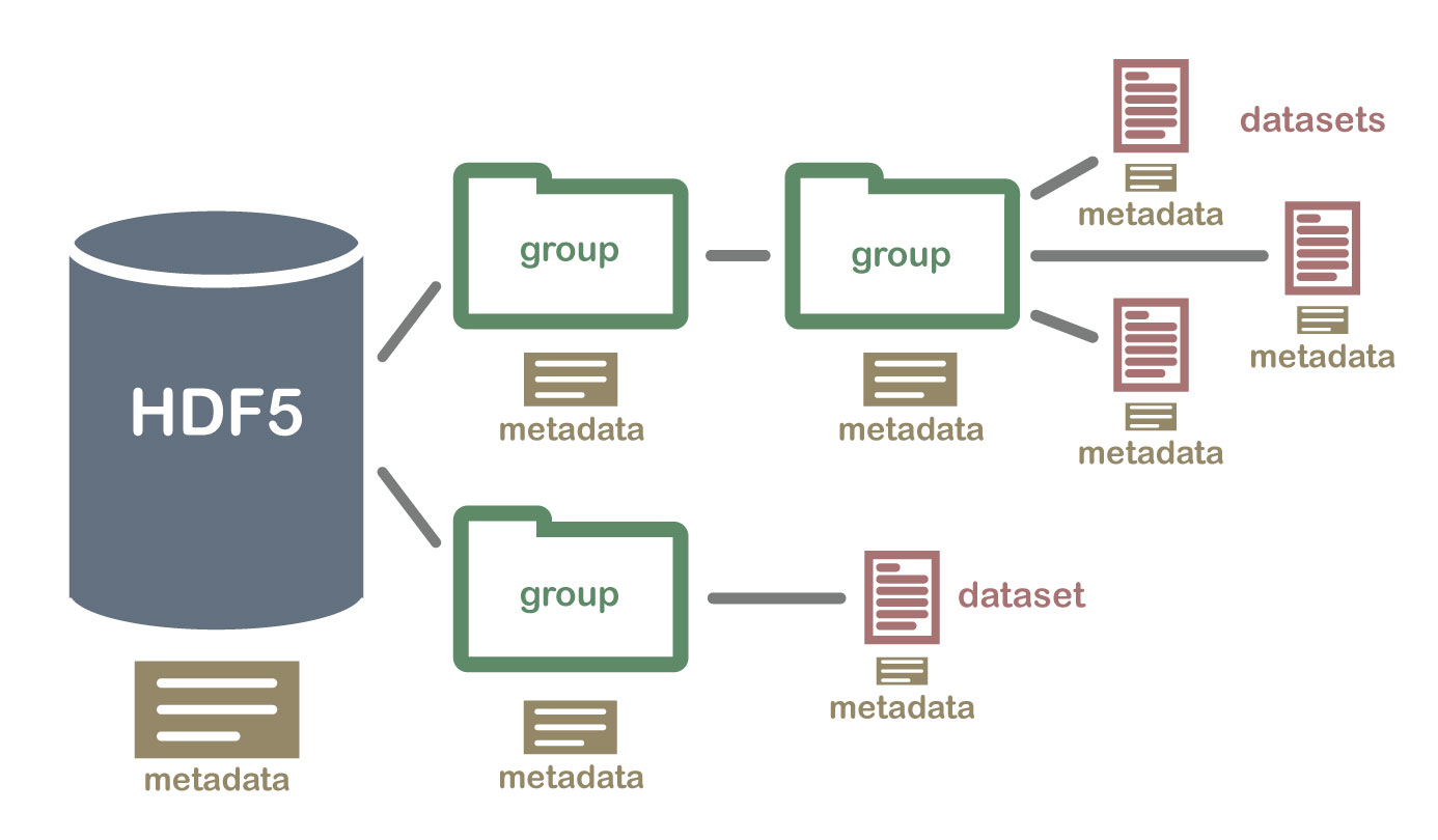 Figure: HDF5 data example. Found in [neonscience](https://www.neonscience.org/resources/learning-hub/tutorials/about-hdf5)
NetCDF
The network Common Data Form, or netCDF, was created in the early 1990s to solve some of the challenges in working with N-dimensional arrays. Netcdf is a collection of self-describing, machine-independent binary data formats and software tools that facilitate the creation, access, and sharing of scientific data stored in N-dimensional arrays, along with metadata describing the contents of each array. Netcdf was built by the climate science community at a time when regional climate models were beginning to produce larger and larger output files. NetCDF version 4 is a subset of HDF5, so netCDF4 files can be opened with HDF5 tools.
Handling large arrays
The netCDF and HDF5 formats have no limit on file size. However, any analysis tool that reads data from a netCDF array into memory for some computational operation is limited by that particular machine’s available memory.
But slow at I/O
When reading a hierarchical file, the whole tree of the data structure is scanned from the root node down. Since this has to be done each time a user makes an inquiry, reading HDF5 and netCDF is slow compared to formats designed for parallel or cloud access.
2.1 Create a dataset and write it to netCDF
We create a synthetic monthly temperature-anomaly field with the course package mlgeo_synth, keep one time slice as a 2D field, and wrap it in an xarray Dataset with coordinates and units.
import mlgeo_synth

field, truth = mlgeo_synth.climate_field(n_lat=40, n_lon=80, n_months=120, seed=42)
print(field.shape)  # (n_months, n_lat, n_lon)
(120, 40, 80)
ds = xr.Dataset(
    data_vars={
        "temperature_anomaly": (
            ("lat", "lon"),
            field[0],
            {"units": "degC", "long_name": "monthly temperature anomaly"},
        )
    },
    coords={
        "lat": ("lat", truth["lat"], {"units": "degrees_north"}),
        "lon": ("lon", truth["lon"], {"units": "degrees_east"}),
    },
    attrs={"title": "Synthetic temperature anomaly, month 0", "source": "mlgeo_synth.climate_field"},
)
dsds.to_netcdf('data/temperature_anomaly.nc')2.2 Read it back with xarray
ds_read = xr.open_dataset('data/temperature_anomaly.nc')
ds_read.temperature_anomaly.plot()
plt.title('Synthetic temperature anomaly (month 0)')
plt.show()
ds_read.close()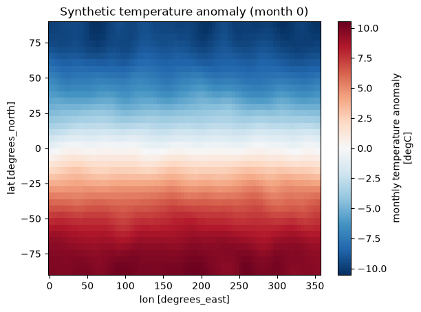
2.3 The same file through the netCDF4 and h5py libraries
The netCDF4 library shows the self-describing structure: dimensions, variables, and attributes.
geo = nc.Dataset('data/temperature_anomaly.nc')
print(geo)
print(geo['temperature_anomaly'])
geo.close()
<class 'netCDF4.Dataset'>
root group (NETCDF4 data model, file format HDF5):
title: Synthetic temperature anomaly, month 0
source: mlgeo_synth.climate_field
dimensions(sizes): lat(40), lon(80)
variables(dimensions): float64 temperature_anomaly(lat, lon), float64 lat(lat), float64 lon(lon)
groups:
<class 'netCDF4.Variable'>
float64 temperature_anomaly(lat, lon)
_FillValue: nan
units: degC
long_name: monthly temperature anomaly
unlimited dimensions:
current shape = (40, 80)
filling on
Because netCDF4 files are HDF5 files, h5py can open the same file. The variables appear as HDF5 datasets, and the metadata as HDF5 attributes.
with h5py.File('data/temperature_anomaly.nc', 'r') as f:
    print("datasets in the root group:", list(f.keys()))
    dset = f['temperature_anomaly']
    print("shape:", dset.shape, "dtype:", dset.dtype)
    print("attributes:", dict(dset.attrs))
datasets in the root group: ['temperature_anomaly', 'lat', 'lon']
shape: (40, 80) dtype: float64
attributes: {'_Netcdf4Coordinates': array([0, 1], dtype=int32), '_FillValue': array([nan]), 'units': np.bytes_(b'degC'), 'long_name': np.bytes_(b'monthly temperature anomaly'), 'DIMENSION_LIST': array([array([<HDF5 object reference>], dtype=object),
array([<HDF5 object reference>], dtype=object)], dtype=object), '_Netcdf4Dimid': np.int32(0)}
3. Zarr
Zarr is a cloud-optimized format for N-dimensional arrays. Instead of a single file, a Zarr store is a directory of compressed chunks plus small JSON metadata files. Cloud object stores and parallel jobs can read individual chunks without scanning the whole file tree, which removes the netCDF/HDF5 I/O bottleneck.
Xarray writes to Zarr directly:
ds.to_zarr('data/temperature_anomaly.zarr', mode='w')/home/runner/work/mlgeo-book/mlgeo-book/.pixi/envs/default/lib/python3.12/site-packages/zarr/api/asynchronous.py:246: ZarrUserWarning: Consolidated metadata is currently not part in the Zarr format 3 specification. It may not be supported by other zarr implementations and may change in the future.
warnings.warn(
<xarray.backends.zarr.ZarrStore at 0x7fd3cf40b7e0>ds_zarr = xr.open_zarr('data/temperature_anomaly.zarr')
ds_zarrThe round trip preserves the data and the metadata:
np.allclose(ds_zarr.temperature_anomaly.values, ds.temperature_anomaly.values)True4. Comparing on-disk sizes across formats
We now store the same data in the formats above and compare their sizes on disk.
- For the table comparison, we flatten the 2D field to a dataframe (one row per grid cell) and write it to CSV and Parquet.
- For the array comparison, we use the netCDF file and the Zarr store we already wrote. A Zarr store is a directory, so we sum the sizes of all files inside it.
# Flatten the array to a table: one row per (lat, lon) grid cell
table = ds.temperature_anomaly.to_dataframe().reset_index()
table.to_csv('data/temperature_anomaly.csv', index=False)
table.to_parquet('data/temperature_anomaly.parquet', index=False)
table.head()def path_size_bytes(path):
"""Size of a file, or the total size of all files under a directory."""
if os.path.isfile(path):
return os.path.getsize(path)
total = 0
for root, _, filenames in os.walk(path):
for filename in filenames:
total += os.path.getsize(os.path.join(root, filename))
return total
sizes = {
'CSV (table)': path_size_bytes('data/temperature_anomaly.csv'),
'Parquet (table)': path_size_bytes('data/temperature_anomaly.parquet'),
'netCDF (array)': path_size_bytes('data/temperature_anomaly.nc'),
'Zarr (array)': path_size_bytes('data/temperature_anomaly.zarr'),
}
comparison = pd.DataFrame(
{'size_kB': [v / 1024 for v in sizes.values()]},
index=sizes.keys(),
).round(1)
print(comparison) size_kB
CSV (table) 133.0
Parquet (table) 33.0
netCDF (array) 33.9
Zarr (array) 29.9
Interpretation: the CSV file is the largest because it stores every number as text, digit by digit. Parquet stores the same table in a compressed binary layout and is several times smaller. The netCDF file and the Zarr store hold the same array in binary form and end up in the same size range; the difference between them at this scale comes from container overhead (HDF5 headers for netCDF, chunk files and JSON metadata for Zarr), not from the data itself. The gap between text and binary formats grows with dataset size, and Zarr’s chunked layout pays off when many processes read different pieces of a large array at once.