Meet the data:
streams, formats, and a first real dataset

Session 4 · Wed Oct 7 · Book sections 2.1–2.2 & 1.6–1.7

🛰️

Today’s question

Every geoscience project ends up handling at least two kinds of data.

Which streams are yours — and what do they deserve to be stored in?

Reading: 2.1 Data definitions · 2.2 Data formats · 1.6 Data gallery · 1.7 GNSS data

Frame the session: Monday was about agents and verification culture; today the course meets its raw material. ML projects in the geosciences succeed or fail on the data, and most of the work is upstream of any model. Two goals for the next 20 minutes: name the three data streams that run through the whole course, and see that a storage format is a scientific decision with measurable consequences — then touch the first real dataset. Ask the room: what data does your intended final project run on? Keep the answers; they map onto today’s table.

This lecture in the literature

📖 The playbook: data that are findable, accessible, interoperable, reusable — what “AI-ready” builds on.

Wilkinson, M. D., et al. (2016). The FAIR Guiding Principles for scientific data management and stewardship. Scientific Data, 3, 160018.

✓ Doing it right: a geoscience paper whose data, provenance, and methods a reader — or a machine — can retrace.

Gil, Y., et al. (2016). Toward the Geoscience Paper of the Future: Best practices for documenting and sharing research from data to software to provenance. Earth and Space Science, 3, 388–415.

✓ Open daily positions for thousands of GNSS stations — the archive today’s P395 series comes from.

Blewitt, G., Hammond, W. C., & Kreemer, C. (2018). Harnessing the GPS data explosion for interdisciplinary science. Eos, 99, doi:10.1029/2018EO104623.

✗ A default file format silently rewrote gene names as dates — corrupting supplementary data across roughly a fifth of surveyed genomics papers.

Ziemann, M., Eren, Y., & El-Osta, A. (2016). Gene name errors are widespread in the scientific literature. Genome Biology, 17, 177.

Data stewardship is published, cited science — and format defaults have corrupted whole literatures.

Two minutes. Wilkinson/FAIR: the 2016 principles — findable, accessible, interoperable, reusable — are the vocabulary funders and journals now require; chapter 2.13’s “AI-ready” checklist is FAIR plus benchmark splits and leakage controls. Gil: what it looks like when a geoscience paper documents data, software, and provenance so the analysis can be retraced — the standard the final project is graded against. Blewitt: the Nevada Geodetic Laboratory processes thousands of permanent GNSS stations and publishes daily positions openly — today’s P395 series is one file of that archive; cite it when you use it. Ziemann: the cautionary tale — spreadsheet software auto-converted gene names like SEPT2 to dates, and the errors sat in the published supplements of roughly a fifth of surveyed genomics papers. A format default, not a scientist, rewrote the data. Refs file updates monthly — bring candidates.

Three data streams run through this course

Stream	Geoscience examples	Shape
Regular high-rate series	100 Hz seismograms, hourly tide gauges, daily GNSS	1D, clocked by the instrument
Gridded fields	climate rasters, satellite imagery, model output	2D–4D arrays over region and time
Irregular sparse points	multi-well networks, field campaigns	samples wherever access allowed

The three get equal treatment in Chapter 2 — because every project ends up handling at least two of them.

This is the chapter’s organizing principle. Walk one example per row: a seismogram is clocked — the instrument fixes the sampling and never misses on purpose; a satellite field is a grid over a region, often with a time axis stacked on; a groundwater network is measured where the wells are and when the crew visits — nothing regular about it. Ask teams to place their project data: most place two streams, which is the point. Preview: sessions 5 and 6 take tables and series/grids in turn; the irregular stream returns Monday with the multi-well network.

Two containers

• Arrays — values on a grid; the dimensions carry the meaning (time, latitude, depth)
• Data frames — one data sample per row, one variable per column; mixed types welcome
• Most projects need both: a gridded field of covariates and a table of observations

Choose the container from the data’s structure, not from the software you opened first.

Define both aloud with a physical example: a 3D array of temperature over latitude, longitude, and time — position in the array IS the coordinate; versus the earthquake catalog — each row one event, columns of time, position, magnitude, text description. Mention modality vocabulary from 2.1 without dwelling: in-situ, remote sensing, model output, geophysical (indirect subsurface). The 2.13 capstone joins the two containers — extracting raster covariates at station locations — so both matter to every team. Implementation names for the notebook, not the slide: NumPy/Xarray for arrays, pandas for data frames.

The same field, on disk

133 kB as CSV — every number spelled out in text

33 kB as Parquet — the same table, typed and compressed

One 40 × 80 temperature-anomaly field, 3,200 grid cells — synthetic (mlgeo_synth), measured in the executed 2.2 notebook.

Text formats store digits; binary formats store numbers. The gap grows with dataset size.

These are the notebook’s own measured numbers — students reproduce them in the exercise. Why the factor of four: CSV writes “9.932382” as eight characters plus separators; Parquet stores an 8-byte float, columnwise, then compresses. At 3,200 cells the gap is 100 kB and nobody cares; at a decade of satellite fields it is the difference between an archive that is usable and one that is not. Also name what CSV throws away: the dtype (everything is text until re-parsed) and the metadata (units live in a README, if anywhere). CSV remains fine for small, human-inspected tables — the course data gallery uses it deliberately.

A format is a set of promises

Format	Built for	Same field on disk
CSV	small tables, human-readable anywhere	133.0 kB
Parquet	large tables — columnar, typed, compressed	33.0 kB
netCDF / HDF5	self-describing arrays: data + units + coordinates in one file	33.9 kB
Zarr	chunked arrays — parallel, partial reads from cloud storage	29.9 kB

The binary formats tie at this size — the difference is what each promises: readability, speed, self-description, or cloud-scale access.

Read the column, then the promises. netCDF: built by the climate community; the file carries its own dimensions, units, and attributes — open it anywhere and it explains itself; netCDF4 is HDF5 underneath (the notebook opens the same file with both libraries). Zarr: not one file but a directory of compressed chunks plus small metadata — a cloud object store can serve a thousand parallel readers each grabbing only their chunk, which is exactly the access pattern netCDF/HDF5 are slow at. Honorable mentions from 2.1 for the notes-curious: GeoTIFF/COG for rasters (the notebook’s Natural Earth relief map — real data), GeoJSON/GeoParquet for vector geometries (the four Cascade volcanoes), STAC for catalogs. Rule of thumb: tables → CSV small / Parquet large; arrays → netCDF local / Zarr cloud.

The first real dataset

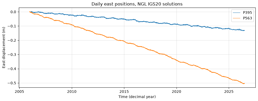
Plate tectonics, measured daily to a few millimeters: GNSS stations P395 & P563 (Pacific Northwest) drift steadily — 7,418 daily solutions at P395 since 2006. Real data — NGL, IGS20 frame.

The course’s first real dataset — savor it. Each point is one daily position solution; the y-axis is east displacement relative to the first day. The smooth drift is plate motion in the IGS20 global reference frame (define: the current international terrestrial reference frame — positions are relative to the whole Earth, so trends are real plate velocities). At P395 the east drift works out to about −6.5 mm/yr — westward — which we will fit, with honest error bars, in section 2.6 on Monday. Look closer: seasonal wiggles from water and snow loading, and small offsets from equipment changes or earthquakes — every later lesson (trend fitting, gap repair, splits) returns to this station. Credit aloud: Nevada Geodetic Laboratory, Blewitt et al. 2018.

Frozen data, living data

• Frozen file (a released dataset): pin its checksum — every future run verifies it got the same bytes
• Living file (NGL appends a new solution daily): pin nothing — log the checksum you actually received
• Publishing or grading? Freeze a snapshot and pin that

Either way, your analysis names its exact input — that is provenance, and it costs one line.

This is 1.6/1.7’s quiet lesson and the habit HW1 grades. Define checksum aloud: a fingerprint of the file’s bytes; if one bit changes, the fingerprint changes. The download tool (pooch, named in the notebook) fetches, caches, and verifies in three lines. The subtlety students hit: a pinned hash on a living file fails tomorrow by design — the file really changed; that failure is information, not a bug. Second habit from 1.6: every dataset carries a license and a citation — carry both forward into your repository. Ask: who can name the license of the data they plan to use? Most cannot — that is this week’s homework moment.

Where each stream lives

Stream	Today’s example	Container	Formats that earn it
Regular high-rate series	P395 daily positions (real, NGL)	time-indexed table / 1D array	CSV small · Parquet, HDF5 at scale
Gridded fields	temperature-anomaly field (synthetic, mlgeo_synth)	labeled array	netCDF local · Zarr cloud
Irregular sparse points	Cascade volcano locations	table + geometry	GeoJSON · GeoParquet

Naming your streams and formats is the first line of your project’s data card — start it today.

The lecture in one screen — leave it up for questions. Each row: the stream (from slide 3), the dataset the students touched or will touch today, the container (slide 4), and format choices with their size/promise trade-offs (slides 5–6). Connect forward: chapter 2 ends with the AI-ready checklist (2.13) and the final-project data assignment (2.20) — a data card documenting exactly these choices plus provenance and licensing. The vocabulary students leave with: stream, container, format, checksum, data card.

Now run it yourself — open 2.2

1. pixi run jupyter lab → 2.2_data_formats_rendered.ipynb
2. Run the round-trips: JSON → CSV/Parquet → GeoTIFF/GeoJSON → netCDF → Zarr; reproduce the size table
3. Open 1.7_get_geodetic_gnss.ipynb: download P395 with pooch, record the SHA256 your run prints
4. Browse the data gallery (1.6): pick one dataset near your project and find its license + citation

Friday: tables that tell the truth (2.3–2.4) · Ch 1 quiz closes Thu Oct 8 · HW1 due Mon Oct 12

Timing for the 80-minute block (10:00–11:20): no pulse talks yet this week — intro and admin ~10 min, deck ~20 min, guided notebook ~40 min, synthesis ~10 min collecting task-4 answers (each team names one dataset, its stream, its license). Implementation names live here and in the notebook: pandas read_csv/to_parquet, rasterio for GeoTIFF, geopandas for GeoJSON, xarray to_netcdf/to_zarr, h5py to peek inside HDF5, pooch.retrieve with known_hash. The Natural Earth raster download is ~100 MB — have neighbors share if the room’s wifi chokes. Remind: Ch 1 quiz closes tomorrow; HW1 (workbench) due Monday; paper-pulse sign-ups are open on Canvas.