3.3 Binary classification

We can compare them all in one exercise.

# Code source: Gaël Varoquaux
#              Andreas Müller
# Modified for documentation by Jaques Grobler
# License: BSD 3 clause

# basic tools
import numpy as np
import matplotlib.pyplot as plt
from matplotlib.colors import ListedColormap
from sklearn.model_selection import train_test_split
from sklearn.preprocessing import StandardScaler
from sklearn.datasets import make_moons, make_circles, make_classification

# classifiers from sklearns
from sklearn.neighbors import KNeighborsClassifier
from sklearn.svm import SVC
from sklearn.gaussian_process import GaussianProcessClassifier
from sklearn.gaussian_process.kernels import RBF
from sklearn.tree import DecisionTreeClassifier
from sklearn.ensemble import RandomForestClassifier, AdaBoostClassifier
from sklearn.naive_bayes import GaussianNB
from sklearn.discriminant_analysis import QuadraticDiscriminantAnalysis

1.1 Synthetic Data

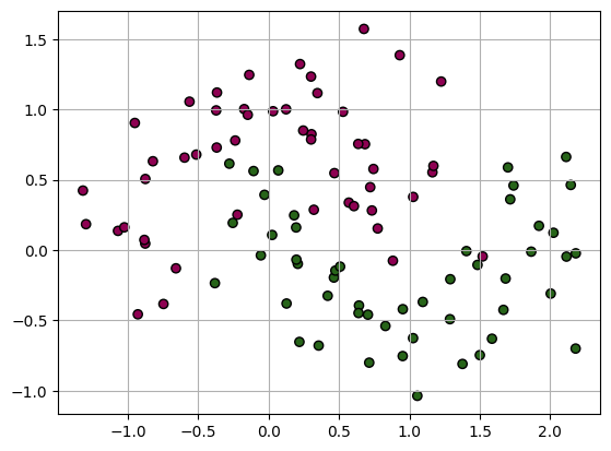
First, we start making new data using the scikitlearn tools.

# make a data set
X, y = make_moons(noise=0.3, random_state=0)

Plot the data

plt.scatter(X[:,0],X[:,1],c=y, cmap='PiYG', edgecolors="k");plt.grid(True)

We will start with the fundamental LDA.

from sklearn.discriminant_analysis import LinearDiscriminantAnalysis

# define ML
clf = LinearDiscriminantAnalysis() 

# normalize data.
X = StandardScaler().fit_transform(X)

# split data between train and test set.
X_train, X_test, y_train, y_test = train_test_split(X, y, test_size=0.4, random_state=42)

# Fit the model.
clf.fit(X_train, y_train)

# calculate the mean accuracy on the given test data and labels.
score = clf.score(X_test, y_test)
print("The mean accuracy on the given test and labels is %f" %score)

The mean accuracy on the given test and labels is 0.875000

from sklearn.inspection import DecisionBoundaryDisplay
ax = plt.subplot()
# plot the decision boundary as a background
DecisionBoundaryDisplay.from_estimator(clf, X, cmap='PiYG', alpha=0.8, ax=ax, eps=0.5)
ax.scatter(X[:, 0], X[:, 1], c=y, cmap='PiYG', alpha=0.6, edgecolors="k")

<matplotlib.collections.PathCollection at 0x7f27e600fd90>

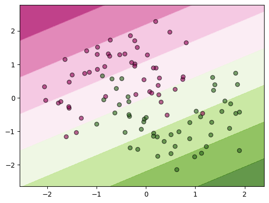
The results shows a not-too bad classification, but a low confidence.

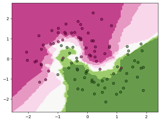
Let’s try a different classifer: KNN

# define ML
K = 5
clf= KNeighborsClassifier(K)

# normalize data.
X = StandardScaler().fit_transform(X)

# split data between train and test set.
X_train, X_test, y_train, y_test = train_test_split(X, y, test_size=0.4, random_state=42)

# Fit the model.
clf.fit(X_train, y_train)

# calculate the mean accuracy on the given test data and labels.
score = clf.score(X_test, y_test)
print("The mean accuracy on the given test and labels is %f" %score)

The mean accuracy on the given test and labels is 0.975000

# plot the decision boundary as a background
ax = plt.subplot()
DecisionBoundaryDisplay.from_estimator(clf, X, cmap='PiYG', alpha=0.8, ax=ax, eps=0.5)
ax.scatter(X[:, 0], X[:, 1], c=y, cmap='PiYG', alpha=0.6, edgecolors="k")

<matplotlib.collections.PathCollection at 0x7f27e3ee9c00>

Now we will test to see what happens when you do not normalize your data before the classification. We will stretch the first axis of the data to see the effects.

# make a data set
X, y = make_moons(noise=0.3, random_state=0)
X[:,0] = 10*X[:,0]
X[:,1] = 10*X[:,1]

# define ML
K = 5
clf= KNeighborsClassifier(K)

# split data between train and test set.
X_train, X_test, y_train, y_test = train_test_split(X, y, test_size=0.4, random_state=42)

# Fit the model.
clf.fit(X_train, y_train)

# calculate the mean accuracy on the given test data and labels.
score = clf.score(X_test, y_test)
print("The mean accuracy on the given test and labels is %f" %score)

# plot the decision boundary as a background
ax = plt.subplot()
# DecisionBoundaryDisplay.from_estimator(clf, X, cmap='PiYG', alpha=0.8, ax=ax, eps=0.5)
ax.scatter(X[:, 0], X[:, 1], c=y, cmap='PiYG', alpha=0.6, edgecolors="k")

The mean accuracy on the given test and labels is 0.975000

<matplotlib.collections.PathCollection at 0x7f27e62d2980>

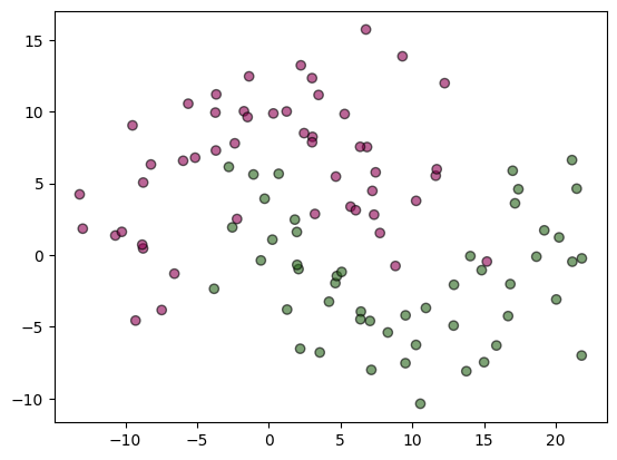
This drastically reduces the performance.

2. Classifier Performance Metrics

In a binary classifier, we label one of the two classes as positive, the other class as negative. Let’s consider N data samples.

True Class \ predicted Class	Positive	Negative	Total
Positive	True Positive	False Negative	p
Negative	False Positive	True Negative	n
Total	p’	n’	N

In this example, there were originally a total of \(p=FN+TP\) positive labels and \(n=FP+TN\) negative levels. We ended up with \(p'=TP+FP\) predicted as positive and \(n'=FN+TN\) predicted as negative.

True positive TP: the number of data predicted as positive that were originally positive.

True negative TN: the number of data predicted as negative that were originally negative.

False positive FP: the number of data predicted as positive but that were originally negative.

False negative FN: the number of data predicted as negative that were originally positive.

Confusion matrix: Count the instances that an element of class A is classified in class B. A 2-class confusion matrix is:

\( C = \begin{array}{|cc|} TP & FN \\ FP & TN \end{array}\)

The confusion matrix can be extended for a multi-class classification and the matrix is KxK instead of 2x2. The best confusion matrix is one that is close to identity, with little off diagonal terms.

Other model performance metrics Model peformance can be assessed with the following:

• Error : the fraction of the data that was misclassified

  \(err = \frac{FP+FN}{N}\) -> 0

• Accuracy: the fraction of the data that was correctly classified:

  \(acc = \frac{TP+TN}{N} = 1 - err \) –> 1

• TP-rate: the ratio of samples predicted in the positive class that are correctly classified:

  \(TPR = \frac{TP}{TP+FN}\) –> 1

  This ratio is also the recall value or sensitivity.

• TN-rate: the ratio of samples predicted in the negative class that are correctly classified:

  \(TNR = \frac{TN}{TN+FP}\) –> 1

  This ratio is also the specificity.

• Precision: the ratio of samples predicted in the positive class that were indeed positive to the total number of samples predicted as positive.

  \(pr = \frac{TP}{TP+FP}\) –> 1

• F1 score:

  \(F_1 = \frac{2}{(1/ precision + 1/recall)} = \frac{TP}{TP + (FN+FP)/2} \) –> 1.

The harmonic mean of the F1 scores gives more weight to low values. F1 score is thus high if both recall and precision are high.

How do precision and recall co-vary?

def returnPrecisionAndRecall(TP, FP, TN, FN):
    precision = TP / (TP + FP) if (TP + FP) else 0
    recall = TP / (TP + FN) if (TP + FN) else 0
    return {'precision': precision, 'recall': recall}

# Okay, set how many true and false values are in the original dataset

actualTrueValues = 50
actualFalseValues = 50

sumValues = 100

precisionRecallCollector = []

# Now, run a set of simulations

for n in range(5000):
    TP = 0
    FP = 0
    TN = 0
    FN = 0
    # Begin by randomly setting the total number of true values returned
    totalTrue = np.random.randint(0, high=sumValues)
    # The total number of false values is sumValues - totalTrue
    totalFalse = sumValues - totalTrue
    # Partition totalTrue and totalFalse into TP, FP and TN, FN, respectively
    if totalTrue != 0:
        TP = np.random.randint(0, high=totalTrue)
        FP = totalTrue - TP
    if totalFalse != 0:
        TN = np.random.randint(0, high=totalFalse)
        FN = totalFalse - TN
    thisPandR = returnPrecisionAndRecall(TP, FP, TN, FN)
    precisionRecallCollector.append([thisPandR['precision'], thisPandR['recall']])

pAndRArray = np.asarray(precisionRecallCollector)
plt.scatter(pAndRArray[:,0], pAndRArray[:,1], color='k', alpha=0.25)
plt.xlabel('Precision')
plt.ylabel('Recall')

From above, we see that a wide range of behavior between precision and recall can be expected. It is not because a classifier might do well in predicting one class than it does predicting the other class. This demonstrates the important of reporting both metrics.

Let’s print these measures from our classification using scikit-learn

from sklearn.metrics import confusion_matrix,precision_score,recall_score,f1_score 

# Fit the model.
y_test_pred=clf.predict(X_test)

print("confusion matrix")
print(confusion_matrix(y_test,y_test_pred))
print("precison, recall")
print(precision_score(y_test,y_test_pred),recall_score(y_test,y_test_pred))
print("F1 score")
print(f1_score(y_test,y_test_pred))

A complete well-formatted report of the performance can be called using the function classification_report:

from sklearn.metrics import classification_report
print(f"Classification report for classifier {clf}:\n"
      f"{classification_report(y_test, y_test_pred)}\n")

Precision and recall trade off: increasing precision reduces recall.

\(precision = \frac{TP}{TP+FP}\)

\(recall = \frac{TP}{TP+FN}\)

The classifier uses a threshold value to decide whether a data belongs to a class. Increasing the threshold gives higher precision score, decreasing the thresholds gives higher recall scores. Let’s look at the various score values.

Receiver Operating Characteristics ROC

It plots the true positive rate against the false positive rate. The ROC curve is visual, but we can quantify the classifier performance using the area under the curve (aka AUC). Ideally, AUC is 1.

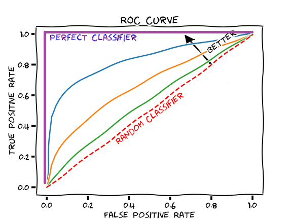
[source: https://commons.wikimedia.org/wiki/File:Roc-draft-xkcd-style.svg]

from sklearn.metrics import roc_curve
from sklearn.model_selection import cross_val_score


y_scores = clf.predict_proba(X_train)
fpr,tpr,thresholds=roc_curve(y_train,y_scores[:,1])
plt.plot(fpr,tpr,linewidth=2);plt.grid(True)
plt.xlabel('False Positive Rate')
plt.ylabel('True Positive Rate')
plt.plot([0,1],[0,1],'k--')

We now explore the different classifiers packaged in scikit learn. We can systematically test their performance and save the precision, recall,

# define models
names = [
    "Nearest Neighbors",
    "Linear SVM",
    "RBF SVM",
    "Gaussian Process",
    "Decision Tree",
    "Random Forest",
    "AdaBoost",
    "Naive Bayes",
    "QDA",
]

classifiers = [
    KNeighborsClassifier(3),
    SVC(kernel="linear", C=0.025),
    SVC(gamma=2, C=1),
    GaussianProcessClassifier(1.0 * RBF(1.0)),
    DecisionTreeClassifier(max_depth=5),
    RandomForestClassifier(max_depth=5, n_estimators=10, max_features=1),
    AdaBoostClassifier(),
    GaussianNB(),
    QuadraticDiscriminantAnalysis(),
]

3. Model exploration

• Explore How each of these models perform on the synthetic data.

• Save in an array the precision, recall, F1 score values.

• Find the best performing model

import pandas as pd
X_train, X_test, y_train, y_test = train_test_split(X, y, test_size=0.4, random_state=42)
pre=np.zeros(len(classifiers))
rec=np.zeros(len(classifiers))
f1=np.zeros(len(classifiers))
for ii,iclass in enumerate(classifiers):
    iclass.fit(X_train, y_train)
    y_test_pred=iclass.predict(X_test)
    pre[ii] =precision_score(y_test,y_test_pred)
    rec[ii] =recall_score(y_test,y_test_pred)
    f1[ii] =f1_score(y_test,y_test_pred)

df=pd.DataFrame({'CLF name':names,'precision':pre,'recall':rec,'f1_score':f1})
print(df)