2.7 Spectral Transforms

Spectral properties of temporal and geospatial data are often important features or signature of a geoscientific event. Filtering the data, or transforming it into a spectral space is a classic feature extraction method in the geosciences.

In this section, we will transform the data by projecting it onto basis of functions. The two most used transforms as the Fourier and the wavelet transforms.

::warning:: Filtering any data needs to be done carefully and potential artefact due to filtering can lead to complete misenterpretation. Awareness for filtering artefacts is very critical for proper scientific investigation. Pitfalls might be

• Not all filters preserve causality: some signals may appear before events and be misinterpreted as precursors.

• Filtering over data gaps brings high frequency artefacts

• Edges effects in filtering times series are difficult to mitigate

The lecture covers several levels and methods for transforming data.

1. Fourier Transforms: basics [Level 1]

2. Fourier Transforms: 2D Fourier transform and Data Compression [Level 3]

3. Short Time Fourier Transforms: spectrograms [Level 2]

4. Wavelet Transforms: basics [Level 3]

# Import modules for seismic data and feature extraction

import numpy as np

import matplotlib.pyplot as plt
import pandas as pd
import scipy
import scipy.signal as signal


# seismic python toolbox
import obspy
import obspy.clients.fdsn.client as fdsn
from obspy import UTCDateTime 

---------------------------------------------------------------------------
ModuleNotFoundError                       Traceback (most recent call last)
/workspaces/mlgeo-instructor/book/Chapter2-DataManipulation/2.7_data_spectral_transforms.ipynb Cell 2 line 1
      <a href='vscode-notebook-cell://codespaces%2Bcurly-winner-7647wqr96rhr49q/workspaces/mlgeo-instructor/book/Chapter2-DataManipulation/2.7_data_spectral_transforms.ipynb#W1sdnNjb2RlLXJlbW90ZQ%3D%3D?line=7'>8</a> import scipy.signal as signal
     <a href='vscode-notebook-cell://codespaces%2Bcurly-winner-7647wqr96rhr49q/workspaces/mlgeo-instructor/book/Chapter2-DataManipulation/2.7_data_spectral_transforms.ipynb#W1sdnNjb2RlLXJlbW90ZQ%3D%3D?line=10'>11</a> # seismic python toolbox
---> <a href='vscode-notebook-cell://codespaces%2Bcurly-winner-7647wqr96rhr49q/workspaces/mlgeo-instructor/book/Chapter2-DataManipulation/2.7_data_spectral_transforms.ipynb#W1sdnNjb2RlLXJlbW90ZQ%3D%3D?line=11'>12</a> import obspy
     <a href='vscode-notebook-cell://codespaces%2Bcurly-winner-7647wqr96rhr49q/workspaces/mlgeo-instructor/book/Chapter2-DataManipulation/2.7_data_spectral_transforms.ipynb#W1sdnNjb2RlLXJlbW90ZQ%3D%3D?line=12'>13</a> import obspy.clients.fdsn.client as fdsn
     <a href='vscode-notebook-cell://codespaces%2Bcurly-winner-7647wqr96rhr49q/workspaces/mlgeo-instructor/book/Chapter2-DataManipulation/2.7_data_spectral_transforms.ipynb#W1sdnNjb2RlLXJlbW90ZQ%3D%3D?line=13'>14</a> from obspy import UTCDateTime 

ModuleNotFoundError: No module named 'obspy'

We will first download data. The seismic data from Puget Sound for a large M8.2 earthquake that happened in Alaska, July 29, 2021.

# Download seismic data
network = 'UW'
station = 'RATT'
channel = 'HHZ'# this channel gives a low frequency, 1Hz signal.
Tstart = UTCDateTime(2021,7,29,6,15)
Tend = Tstart+7200# UTCDateTime(year=2022, month=10, day=8)
fdsn_client = fdsn.Client('IRIS') # client to query the IRIS DMC server

# call to download the specific data: earthquake waveforms
Z = fdsn_client.get_waveforms(network=network, station=station, location='--', channel=channel, starttime=Tstart, \
    endtime=Tend, attach_response=True)
# basic pre-processing: merge all data if there is gaps, detrend, taper,
#  remove the seismic instrumental response to go from the digitizer units to ground motion (velocity) units.
Z.merge(); Z.detrend(type='linear'); Z[0].taper(max_percentage=0.05)


# call to download the specific data: noise waveforms
N = fdsn_client.get_waveforms(network=network, station=station, location='--', channel=channel, starttime=Tstart-7200, \
    endtime=Tstart, attach_response=True)
# basic pre-processing: merge all data if there is gaps, detrend, taper,
#  remove the seismic instrumental response to go from the digitizer units to ground motion (velocity) units.

N.merge(); N.detrend(type='linear');N[0].taper(max_percentage=0.05)

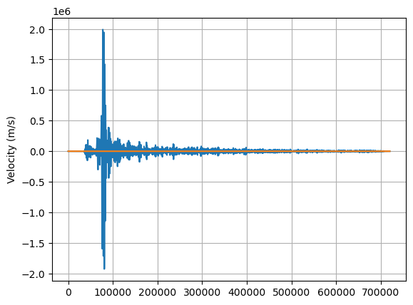
UW.RATT..HHZ | 2021-07-29T04:15:00.000000Z - 2021-07-29T06:14:59.990000Z | 100.0 Hz, 720000 samples

plt.plot(Z[0].data);plt.plot(N[0].data);plt.grid(True);plt.ylabel('Velocity (m/s)')

Text(0, 0.5, 'Velocity (m/s)')

1. Fourier Transforms [Level 1]

We use the Scipy Fourier package to transform the two time series (earthquake and noise).

The Fourier transform is a decomposition of the time series onto an orthonormal basis of cosine and sine functions. The Fourier transform of a time series \(f(t)\) (but similarly if the variable is space \(x\)).

\(\hat{F}(f) = \int_{-\infty}^\infty f(t) \exp^{-i2\pi ft} dt\)

\(\hat{F}(f)\) is the complex Fourier value at frequency \(f\). The Fourier transform determines what frequency(ies) dominate the time series.

1.1 Nyquist

The Fourier transform we will use in this class takes a discrete time series of real numbers. The time series is sampled with \(N\) samples per seconds. If the time series span \(T\) seconds regularly, then the sampling rate of the data \(dt=T/N\). The highest frequency that can be resolved in a discrete time series, called the Nyquist frequency, is limited by \(dt\):

\(F_{Nyq} = \frac{1}{2dt N}\)

Effectively, one cannot constrain signals within two time samples from the data.

1.2 Uncertainties

• The discrete Fourier Transform yields an approximation of the FT. The shorter the time series, the least accurate is the FT. This means that the FT on short time windows is less accurate

• The FT assumes (and requires) the periodicity of the series, meaning that the finite/trimmed time series would repeat in time. To enforce this, we taper the time series so that the first and last points are equal (to zero).

from scipy.fftpack import fft, ifft, fftfreq, next_fast_len

npts = Z[0].stats.npts
## FFT the signals
# fill up until 2^N value to speed up the FFT
Nfft = next_fast_len(int(Z[0].data.shape[0])) # this will be an even number
freqVec = fftfreq(Nfft, d=Z[0].stats.delta)[:Nfft//2]
Z.taper(max_percentage=0.05)
Zhat = fft(Z[0].data,n=Nfft)#/np.sqrt(Z[0].stats.npts)

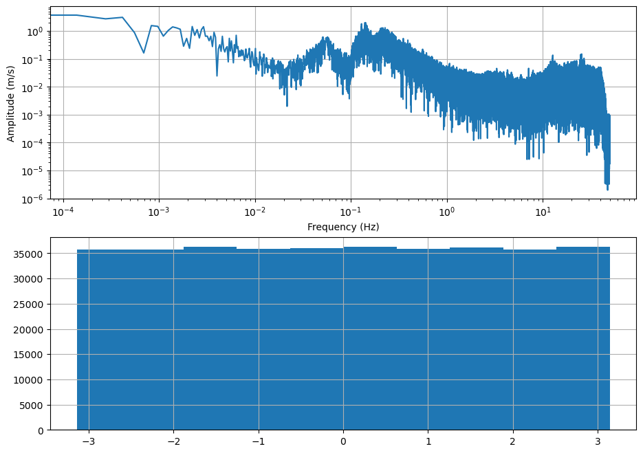
Please see the Obspy documentation to find out about the taper function. Plot the amplitude and phase spectra

fig,ax=plt.subplots(2,1,figsize=(11,8))
ax[0].plot(freqVec,np.abs(Zhat[:Nfft//2])/Nfft)
ax[0].grid(True)
ax[0].set_xscale('log');ax[0].set_yscale('log')
ax[0].set_xlabel('Frequency (Hz)');ax[0].set_ylabel('Amplitude (m/s)')
ax[1].hist(np.angle(Zhat))
ax[1].grid(True)

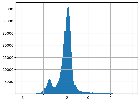
You will note above that the phase values are randomly distributed between \(-\pi\) and \(\pi\). We can check it by showing the distribution of the phase and amplitude spectra.

# your turn. Plot the histograms of the phase and amplitude spectrum
plt.hist(np.log10(np.abs(Zhat[:Nfft//2])/Nfft),100);plt.grid(True)
plt.show()

We can also analyze the spectral characteristics of the noise time series. Below,

1. compute the Fourier transform

2. plot the phase and amplitude spectra

3. plot the distribution of the phase and amplitude values

# compute Fourier transform of the noise time series

npts1 = N[0].stats.npts
## FFT the signals
# fill up until 2^N value to speed up the FFT
Nfft1 = next_fast_len(int(N[0].data.shape[0])) # this will be an even number
freqVec1 = fftfreq(Nfft1, d=N[0].stats.delta)[:Nfft1//2]

# taper the data to enable periodicity
N.taper(max_percentage=0.05)

# Fourier transform
Nhat = fft(N[0].data,n=Nfft1)#/np.sqrt(Z[0].stats.npts)

# plot the phase and amplitude spectra
fig,ax=plt.subplots(2,1,figsize=(11,8))
ax[0].plot(freqVec1,np.abs(Nhat[:Nfft1//2])/Nfft1)
ax[0].grid(True)
ax[0].set_xscale('log');ax[0].set_yscale('log')
ax[0].set_xlabel('Frequency (Hz)');ax[0].set_ylabel('Amplitude (m/s)')
ax[1].hist(np.angle(Nhat[:Nfft1//2]))
ax[1].grid(True)

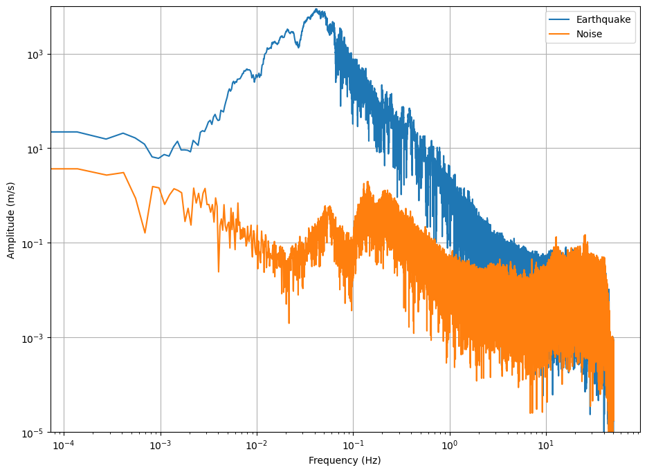
# Overlay the spectrum of the data and the spectrum of the noise

fig,ax=plt.subplots(1,1,figsize=(11,8))
ax.plot(freqVec,np.abs(Zhat[:Nfft//2])/Nfft)
ax.plot(freqVec1,np.abs(Nhat[:Nfft1//2])/Nfft1)
ax.grid(True)
ax.set_xscale('log');ax.set_yscale('log')
ax.set_xlabel('Frequency (Hz)');ax.set_ylabel('Amplitude (m/s)')
ax.legend(['Earthquake','Noise'])
ax.set_ylim([1e-5,1e4])

(1e-05, 10000.0)

Overlay their PDFs

# your turn. Plot the histograms of the phase and amplitude spectrum
plt.hist(np.log10(np.abs(Zhat[:Nfft//2])/Nfft),100)
plt.hist(np.log10(np.abs(Nhat[:Nfft1//2])/Nfft1),100)
plt.grid(True)
plt.show()

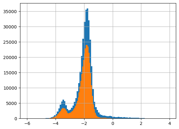
You notice that their statistical differences are in the tails of the distributions. Therefore, statistical metrics such as mean or variance may not be discriminatory, but kurtosis might.

print("Skewness")
print(scipy.stats.skew(np.log10(np.abs(Zhat[:Nfft//2]))),
scipy.stats.skew(np.log10(np.abs(Nhat[:Nfft1//2]))))

print("Kurtosis")
print(scipy.stats.kurtosis(np.log10(np.abs(Zhat[:Nfft//2]))),
scipy.stats.kurtosis(np.log10(np.abs(Nhat[:Nfft1//2]))))

print("mean")
print(np.mean(np.log10(np.abs(Zhat[:Nfft//2]))),
np.mean(np.log10(np.abs(Nhat[:Nfft1//2]))))

print("standard deviation")
print(np.std(np.log10(np.abs(Zhat[:Nfft//2]))),
np.std(np.log10(np.abs(Nhat[:Nfft1//2]))))

Skewness
0.8453316591120342 -1.2201005948153714
Kurtosis
6.236217054087575 1.6480666066247558
mean
3.8679961043240163 3.767943601369907
standard deviation
0.8309308755379773 0.6173489951795071

1.3 Filtering in the Fourier space

The data may superimpose multiple signals of various frequencies. To remove or extract specific signals that do not overlap in frequencies, we can filter the data.

The filter can be:

• high pass: reduce signals at frequencies lower than a corner frequency \(f_c\), only let the signals above \(f_c\). Often parameterized in functions as hp or highpass.

• low pass: reduce signals at frequencies greater than a cutoff frequency \(f_c\), only let the signals below that \(f_c\). Often parameterized in functions as lp or lowpass.

• band pass: reduce signals at frequencies lower than a low corner frequency \(f_{c1}\) and at frequencies greater than a high corner frequency \(f_{c2}>f_{c1}\). Often parameterized as bp or bandpass.

There exist different types of filters, the most common are butterworth and chebyshev, but there exist others.

Examples of filters illustrated here.

One example is that we want to remove unrealistic signals arising from sensor limitations. Seismometers are rarely sensitive to signals that have periods longer than 100s.

We will use the scipy.signal module to filter the time series. First we remove the unrealistic signals past 150 s.

# sampling rate of the data:
fs = Z[0].stats.sampling_rate
z=np.asarray(Z[0].data)
n=np.asarray(N[0].data)

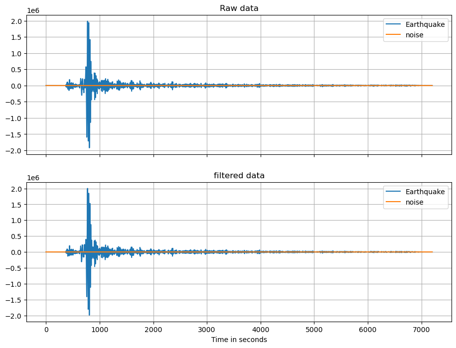
We use here a butterworth filter of second order between 1s and 150s. The sos filter is a second-order sections, which are the product of second-order polynomials to represent the original filters. They are more complex but more stable.

sos = signal.butter(2,[1./150.,1.], 'bp', fs=fs, output='sos')
zf = signal.sosfilt(sos, z)
nf = signal.sosfilt(sos, n)
t=np.arange(0.,7200.,1./fs)

fig,ax=plt.subplots(2,1,figsize=(11,8),sharex=True)
ax[0].plot(t,z[:-1]);ax[0].plot(t,n);ax[0].grid(True)
ax[0].set_title('Raw data');ax[0].legend(['Earthquake','noise'])
ax[1].plot(t,zf[:-1]);ax[1].plot(t,nf);ax[1].grid(True)
ax[1].set_title('filtered data');ax[1].legend(['Earthquake','noise'])
ax[1].set_xlabel('Time in seconds')

Text(0.5, 0, 'Time in seconds')

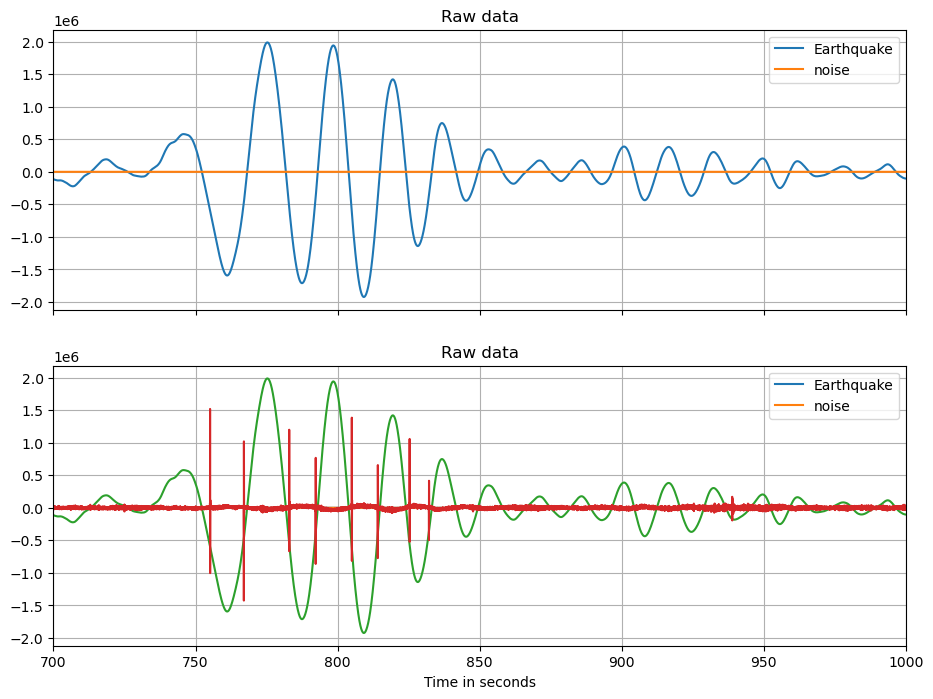
Now filter at high frequencies (>10Hz) and compare earthquakes and noise signals.

# enter below

sos = signal.butter(2,[10,40.], 'bp', fs=fs, output='sos')
zf = signal.sosfilt(sos, z)
nf = signal.sosfilt(sos, n)
t=np.arange(0.,7200.,1./fs)

fig,ax=plt.subplots(2,1,figsize=(11,8),sharex=True)
ax[0].plot(t,z[:-1]);ax[0].plot(t,n);ax[0].grid(True)
ax[0].set_title('Raw data');ax[0].legend(['Earthquake','noise'])
ax[1].plot(t,zf[:-1]);ax[1].plot(t,nf);ax[1].grid(True)
ax[1].set_title('filtered data');ax[1].legend(['Earthquake','noise'])
ax[1].set_xlabel('Time in seconds')
ax[0].set_xlim([700,1000])
ax[1].set_xlim([700,1000])


plt.plot(t,z[:-1]);plt.grid(True)
plt.title('Raw data');plt.legend(['Earthquake','noise'])
plt.plot(t,zf[:-1]*1000)
plt.xlabel('Time in seconds')
plt.xlim([700,1000])

(700.0, 1000.0)

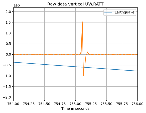
plt.plot(t,z[:-1]);plt.grid(True)
plt.title('Raw data vertical UW.RATT');plt.legend(['Earthquake','noise'])
plt.plot(t,zf[:-1]*1000)
plt.xlabel('Time in seconds')
plt.xlim([754,756])

(754.0, 756.0)

2. 2D Fourier Transforms [Level 3]

The 2D Fourier transform is applied on a 2D matrix. It first applies a 1D Fourier transform to every row of the matrix, then applies a 1D Fourier transform to every column of the intermediate matrix.

2D Fourier transforms can be used to find the Fourier coefficients that dominate the image. This can be used for filtering the data. Another application is to compress the data by selecting several coefficients instead of presenting most of the image.

We will practice on a DEM.

!pip install wget
import wget
import os
import netCDF4 as nc

Collecting wget
  Using cached wget-3.2-py3-none-any.whl
Installing collected packages: wget
Successfully installed wget-3.2

# Download the geological framework
file1 = wget.download("https://www.dropbox.com/s/wdb25puxh3u07dj/NCM_GeologicFrameworkGrids.nc?dl=1") #"./data/NCM_GeologicFrameworkGrids.nc"
# Download the coordinate grids
file2 = wget.download("https://www.dropbox.com/s/i6tv3ug15oe6yhe/NCM_SpatialGrid.nc?dl=1") #"./data/NCM_GeologicFrameworkGrids.nc"

# read data
geology = nc.Dataset(file1)
grid = nc.Dataset(file2)

# create a grid of latitude and longitude
x = grid['x'][0:4901, 0:3201]
y = grid['y'][0:4901, 0:3201]
elevation = geology['Surface Elevation'][0:4901, 0:3201]
plt.contourf(x, y, elevation)

# recreate the lat long vectors.
minlat,maxlat = min(grid['Latitude vector'][:]),max(grid['Latitude vector'][:])
minlon,maxlon = min(grid['Longitude vector'][:]),max(grid['Longitude vector'][:])
xlat = np.linspace(minlat,maxlat,3201)
xlon = np.linspace(minlon,maxlon,4901)

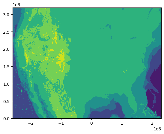
Consider elevation as a 2D data set. We can perform a 2D transform, which will give us a spectrum in the spatial dimension.

from scipy.fftpack import fft2, fftfreq,fftshift, ifft2
import matplotlib.cm as cm
Zel = fft2(elevation)



# make a vector of distances. Here I will ignore the curvature and spatial projection.
# make the wavenumber frequency vector: 
Rlon = (xlon-np.min(xlon))*111.25  # convert degrees to kms
drlon = Rlon[1]-Rlon[0]
print("this is about the spatial sampling of the model ",drlon," km")
klon = (fftfreq( 4901//2 , drlon  ))


Rlat = (xlat-np.min(xlat))*111.25  # convert degrees to kms
drlat = Rlat[1]-Rlat[0]
print("this is about the spatial sampling of the model ",drlat," km")
klat = (fftfreq( 3201//2 , drlat  ))

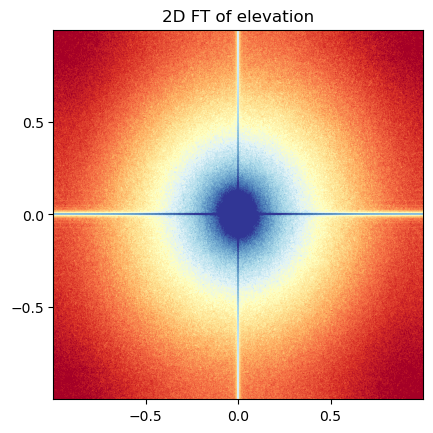
# amplitude of the DEM
plt.imshow(fftshift(np.log10(np.abs(Zel)/Zel.size)),vmin=-3, vmax=-1, cmap='RdYlBu',extent=[-1,1,-1,1])
plt.title('2D FT of elevation')
x_label_list = ['-1/3 km$^{-1}$','0','1/3  km$^{-1}$']
plt.xticks([-0.5,0,0.5])
plt.yticks([-0.5,0,0.5])
plt.show()

this is about the spatial sampling of the model  1.5007397612756534  km
this is about the spatial sampling of the model  1.0777344413103096  km

Now we will filter or compress by taking the largest Fourier coefficients of the image.

# Sort the Fourier coefficients
Zsort = np.sort(np.abs(np.abs(Zel).reshape(-1)))

print(len(Zsort))
print(Zsort.shape)

15688101
(15688101,)

from IPython import display
import time
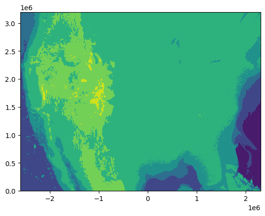
for keep in (0.1,0.05,0.01):
    display.clear_output(wait=True)
    thresh = Zsort[int(np.floor( (1-keep)*len(Zsort) ))]
    ind = np.abs(Zel)>thresh
    Atlow = Zel * ind # here we zero out the matrix
    # Here we count the number of non-zeros in the matrix
    print("We are keeping up to %f the number of Fourier coefficients" % keep)
    Alow = ifft2(Atlow).real
    plt.contourf(x, y, Alow)
    time.sleep(1)

We are keeping up to 0.010000 the number of Fourier coefficients

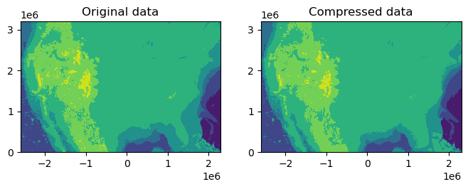
Now we will compare the original 2D data set with the Fourier compressed data

keep=0.01
thresh = Zsort[int(np.floor( (1-keep)*len(Zsort) ))]
ind = np.abs(Zel)>thresh
Atlow = Zel * ind # here we zero out the matrix
# Here we count the number of non-zeros in the matrix
print("We are keeping up to %f the number of Fourier coefficients" % keep)
Alow = ifft2(Atlow).real


fig,ax=plt.subplots(1,2,figsize=(8,8),sharex=True)
ax[0].contourf(x, y, elevation);ax[0].set_title('Original data')
ax[0].axis('scaled')
ax[1].contourf(x, y, Alow);ax[1].set_title('Compressed data')
ax[1].axis('scaled')

We are keeping up to 0.010000 the number of Fourier coefficients

(-2600000.0, 2300000.0, 0.0, 3200000.0)

3. Short Time Fourier Transforms [Level 2]

In time-dependent and multi-scale problems, it may be interesting to extract data features from the short time Fourier transform.

The STFT is a Fourier Transform applied to short (overlapping) windows to resolve the frequencies over different times in the series.

from scipy.signal import stft

nperseg=1000
z=np.asarray(Z[0].data)
f, t, Zxx = stft(z, fs=100, nperseg=nperseg,noverlap=200)
print(np.max(np.max(np.abs(Zxx))))
fig,ax=plt.subplots(2,1,figsize=(11,8),sharex=True)
ax[0].pcolormesh(t/3600, f, np.log10(np.abs(Zxx)), vmin=-1, vmax=3.5, shading='gouraud')
ax[0].set_title('STFT Magnitude')
ax[0].set_ylabel('Frequency [Hz]')
# ax[0].set_xlabel('Time [Hours]')
ax[0].set_yscale('log');ax[0].set_ylim(0.1,40)


n=np.asarray(N[0].data)
f, t, Zxx = stft(n, fs=100, nperseg=nperseg,noverlap=200)
print(np.max(np.max(np.abs(Zxx))))
ax[1].pcolormesh(t/3600, f, np.log10(np.abs(Zxx)), vmin=-1, vmax=0.5, shading='gouraud')
# ax[1].set_title('Noise Magnitude')
ax[1].set_ylabel('Frequency [Hz]')
ax[1].set_xlabel('Time [Hours]');ax[1].set_yscale('log');ax[1].set_ylim(0.1,40)

1767563.2884356107
47.86349029869899

/var/folders/js/lzmy975n0l5bjbmr9db291m00000gn/T/ipykernel_47043/1691094658.py:8: RuntimeWarning: divide by zero encountered in log10
  ax[0].pcolormesh(t/3600, f, np.log10(np.abs(Zxx)), vmin=-1, vmax=3.5, shading='gouraud')

(0.1, 40)

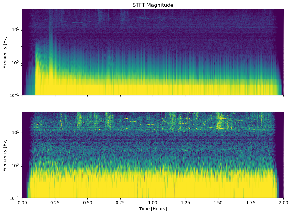
The spectrogram Zxx is a transform of the original data. It is common to use spectrograms as input to neural networks as 2D arrays.

Zxx.shape

(501, 901)

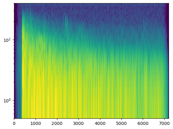
4. Wavelet Transforms: basics [Level 2]

The wavelet transform projects the time series onto a 2D space of time and scale axis. The scale is a representation of the frequency scale of the data. The wavelet transforms uses a series of functions called wavelets to linearly decompose the signals. Unlike the sine functions of the Fourier transform, the wavelets have finite durations and are localized in time:

Image from this article.

There exist many canonical wavelet families. The difference between families is typically their shape, compactness, and smoothness. Typically, one chooses one family for the specific time series. Wavelets have finite energy and zero mean.

The time-scale representation of a time series is a scaleogram. scales can be converted to pseudo frequencies: If \(f_c\) is the central frequency of the wavelet and the scale is \(a\), then the pseuo-frequency is \(f_a = f_c/a\).

Image from this article.

The wavelet transform becomes:

\(\hat{F}(a,b) = \frac{1}{\sqrt{a}} \int_{-\infty}^\infty f(t) \bar{\Psi} (\frac{t-b}{a}) dt\)

where \(\bar{\Psi}\) is the mother wavelet scaled by a factor of \(a\) and translated/shifted by \(b\). The wavelet transform is scaled by the continuous and “infinite number of values” of \(a\) and \(b\) are continuous. The Discrete Wavelet Transform is the wavelet transform performed on a finite number of scales and shifts.

import scipy.signal as signal


t = np.arange(0,(Tend-Tstart)+Z[0].stats.delta,Z[0].stats.delta)
fs=1/Z[0].stats.delta

# use the number of scales
w = 6.

# relate scales with frequencies
# freq = np.linspace(0, fs/2, 100)
freq = np.logspace(-1, np.log10(fs/2), 100)
widths = w*fs / (2*freq*np.pi)


cwtm = signal.cwt(z, signal.morlet2, widths, w=w)

Calculating the time-frequency representation of large time series

# cwtmatr = signal.cwt(z, signal.morlet, widths)
plt.imshow(np.log10(np.abs(cwtm)), extent=[t.min(),t.max(),freq.min(),freq.max()], cmap='viridis', aspect='auto',
           vmax=6, vmin=-0.5,origin='lower')
plt.yscale('log')
plt.ylim([0.5,40])
plt.show()

TF transforms take computational time in the workflow, let’s compare:

%timeit cwtm = signal.cwt(z, signal.morlet2, widths, w=w)
%timeit f, t, Zxx = stft(n, fs=100, nperseg=nperseg,noverlap=200)

5.51 s ± 26.5 ms per loop (mean ± std. dev. of 7 runs, 1 loop each)
5.5 ms ± 166 µs per loop (mean ± std. dev. of 7 runs, 100 loops each)

From these transform, we can extract similar statistical features