2.6 Resampling Methods
Contents
2.6 Resampling Methods#
Data have natural variability, which we often have to account for.
Among other applications (e.g., uncertainity propagation or assigning confidence intervals to some statistic), resampling methods can help us explore this varaibility.
Broadly, resampling refers to any technique where we repeatedly draw observations from some sample.
The lecture introduces resampling techniques in several ways. We explore various fundamental examples of resampling (Level 1) and demonstrate how resampling can be used for model inference of a linear regression (Level 2).
First of all, import some useful modules:
import requests, zipfile, io, gzip, glob, os
import matplotlib.pyplot as plt
import numpy as np
import pandas as pd
%matplotlib inline
# fix the random seed for reproducibility. Place it on the top to reproduce the entire notebook exactly once. But use it in every cell to re-run each cells independently.
np.random.seed(42)
# We define a random generator
rng = np.random.default_rng()
rng
Generator(PCG64) at 0x7F9CEA70FE60
1. Examples of resampling techniques (Level 1)#
1.1 Randomization#
As we introduced in class:
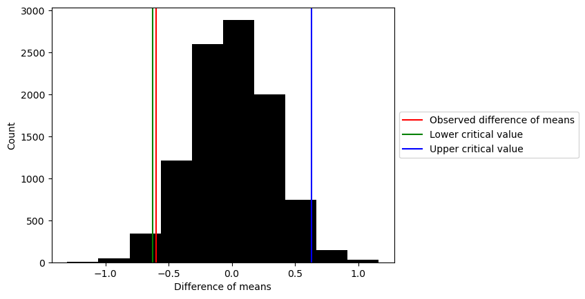
Given two datasets, \(A\) and \(B\), and a parameter, \(x\), we can randomly assign observations to either \(A\) or \(B\), calculate some statistic (e.g., \(x_A - x_B\)), and repeat to build a distribution of that statistic.
# We begin with two datasets, A and B
np.random.seed(42)
rng = np.random.default_rng(seed=42)
A = rng.normal(5, 2.5, 100)
B = rng.normal(5.5, 2.5, 100)

# We then calculate the means of each dataset
mean_A = np.mean(A)
mean_B = np.mean(B)

print('The means of A and B are, ' + str(mean_A) + ' and ' + str(mean_B) + ', respectively.')

# And, for the sake of illustration, also calculate the difference between these means

diff_means = mean_A - mean_B

print('The difference of means is, ' + str(diff_means) + '.')
The means of A and B are, 4.874325971290356 and 5.473420405447642, respectively.
The difference of means is, -0.5990944341572852.
Now, we will want to resample.
# First, how many times do we want to resample?
number_runs = 10000
# Next, we create an array that will store the difference of means
array_of_diffs = np.zeros([number_runs, 1])
# To ease computational burden, let's declare some variables
# A combined list of A and B
combined = np.concatenate((A, B))
# Length of A and B
length_A = len(A)
For each time we resample, we recalculate the mean and recalculate the difference
# For each run:
for i in range(number_runs):
    # Let us shuffle the combined list
    # Note that shuffle works in place!
    rng.shuffle(combined)
    # Now, split the list into A and B, maintaining their original sizes
    # Notice the slice syntax!
    new_A = combined[0:length_A]
    new_B = combined[length_A:len(combined)]
    # Calculate and store a difference of means
    array_of_diffs[i] = np.mean(new_A) - np.mean(new_B)
# Plot up the array of diffs
plt.hist(array_of_diffs, color='black')

# Given an alpha of 0.05, can we accept or reject the null hypothesis of no difference in means?

alpha = 0.05
lower_critical_value = np.quantile(array_of_diffs, alpha/2)
upper_critical_value = np.quantile(array_of_diffs, 1-(alpha/2))

# Plot the critical values and the observed value
plt.axvline(x = diff_means, color='r')
plt.axvline(x = lower_critical_value, color='g')
plt.axvline(x = upper_critical_value, color='b')
plt.xlabel('Difference of means')
plt.ylabel('Count')
plt.legend(['Observed difference of means', 'Lower critical value', 'Upper critical value'], loc='center left', bbox_to_anchor=(1, 0.5))
# Show your plot
plt.show()
1.2 Bootstrapping#
When bootstrapping, you repeatedly draw observations, with replacement, from a dataset. Since you are drawing with replacement, your newly resampled dataset likely will contain duplicate observations from the original sample.
Bootstrapping does not make strong assumptions about the underlying distribution of the dataset.
We will first create correlated data using the numpy function random.multivariate_normal (docs here). The mean of both data will be zero and their covariance is -0.75.
# We begin with a dataset where two variables are strongly correlated
correlated_data= np.random.multivariate_normal([0, 0], [[1, -.75], [-.75, 1]], 1000)
First, we check that the data is indeed anticorrelated by plotting one against the other
plt.scatter(correlated_data[:, 0], correlated_data[:, 1], marker='x', c='black')
plt.xlabel('X')
plt.ylabel('Y')
plt.legend(['Observation'])
plt.show()
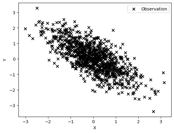
We can verify that the Pearson correlation coefficient is close to our target using the numpy function corrcoef.
# The correlation matrix of the first and second columns of correlated_data
correlation_matrix = np.corrcoef(correlated_data[:, 0], correlated_data[:, 1])
correlation_matrix
array([[ 1.        , -0.72540304],
       [-0.72540304,  1.        ]])
# Check the correlation coefficient
print('The correlation coefficient is: ' + str(correlation_matrix[0,1]) + '.')
The correlation coefficient is: -0.7254030411293305.
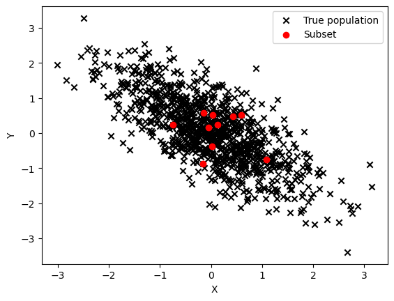
We now take a subset of the data — think of the subset as a sample of the true population.
nsubset=10
subset = rng.choice(correlated_data, size=nsubset, replace=True)
subset
array([[ 1.08149552, -0.75473902],
       [-0.15064708, -0.88421426],
       [ 0.03331803,  0.51951422],
       [ 0.58669726,  0.51967288],
       [ 0.42511267,  0.47888931],
       [-0.05371048,  0.15998988],
       [ 0.13428352,  0.24026582],
       [-0.13976786,  0.57151718],
       [-0.74081486,  0.22763649],
       [ 0.02037839, -0.36898269]])
We can calculate the correlation coefficent of this sample.
# Report the correlation coefficient of the subset
print('The correlation coefficient of our sample is: ' + str(np.corrcoef(subset[:,0], subset[:, 1])[0,1]) + '.')

# Plot up both the original data and our sample
plt.scatter(correlated_data[:, 0], correlated_data[:, 1], marker='x', c='black')
plt.scatter(subset[:,0], subset[:, 1], c='red')
plt.xlabel('X')
plt.ylabel('Y')
plt.legend(['True population', 'Subset'])
plt.show()
The correlation coefficient of our sample is: -0.19742697173045343.
Now, we will bootstrap. Once again, we define a number of runs.
number_runs =1000
Each time we resample, we will calculate and store the correlation coefficent of the resampled data.
# Create an array that will keep track of the outputs of our resampling loop. In this case, we just want to record the correlation coefficient of each new sample.
corr_coef_collector = np.zeros([number_runs, 1])

# Let's also get the length of the subset
# When bootstrapping, the size of your resampled dataset should match the size of your original sample!
length_sub = len(subset)
length_sub = 100
subset
array([[ 1.08149552, -0.75473902],
       [-0.15064708, -0.88421426],
       [ 0.03331803,  0.51951422],
       [ 0.58669726,  0.51967288],
       [ 0.42511267,  0.47888931],
       [-0.05371048,  0.15998988],
       [ 0.13428352,  0.24026582],
       [-0.13976786,  0.57151718],
       [-0.74081486,  0.22763649],
       [ 0.02037839, -0.36898269]])
nsubset=10

subset
array([[ 1.08149552, -0.75473902],
       [-0.15064708, -0.88421426],
       [ 0.03331803,  0.51951422],
       [ 0.58669726,  0.51967288],
       [ 0.42511267,  0.47888931],
       [-0.05371048,  0.15998988],
       [ 0.13428352,  0.24026582],
       [-0.13976786,  0.57151718],
       [-0.74081486,  0.22763649],
       [ 0.02037839, -0.36898269]])
nsubset=500
# Now, for each run
for i in range(number_runs):
    # We want to draw length_sub samples WITH REPLACEMENT
    new_pairs = rng.choice(correlated_data, size=nsubset, replace=True)
    # Calculate and store the correlation coefficient
    corr_coef_collector[i] = np.corrcoef(new_pairs[:, 0], new_pairs[:, 1])[0,1]

# Plot up the corr_coef_collector values
plt.hist(corr_coef_collector, color='black')
plt.xlabel('Correlation coefficient')
plt.ylabel('Count')

# Show the true correlation coefficient
plt.axvline(x=correlation_matrix[0,1], color='red')
plt.axvline(x=np.median(corr_coef_collector), color='blue')
plt.legend(['True correlation coefficient', 'Median correlation coefficient'])
plt.show()
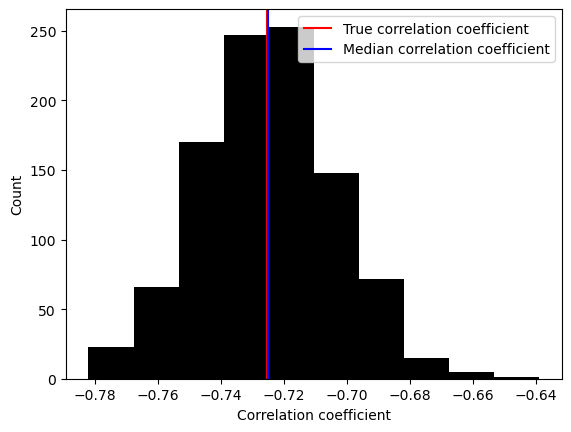
We see that the median Pearson coefficient is not exactly the true Pearson coefficient. Why is that?
What happens if you increase the size of the subset (e.g., your sample of the true population)?
1.3 Monte Carlo#
Named after the casino in Monaco, Monte Carlo methods involve simulating new data based on a known (or assumed!) statistical model. Unlike the previous two examples, we do not take draws from an existing sample.
Monte Carlo techniques have many applications. For example, you might see Monte Carlo methods used for probabilistic risk assessment, uncertainty propagation in models, and evaluating complex systems’ performance. It is especially valuable when dealing with complex geospatial, environmental, or engineering models, where the relationships among variables are not easily captured by simple parametric methods.
Here, we demonstrate Monte Carlo sampling by trying to estimate \(\pi\).
We begin with a central conceit: that the ratio of the area of a circle to the area of the square is \(\pi/4\).
We then imagine a circle of radius 1 that is inscribed within a square with sides going from -1 to 1.
# We're going to draw a (x,y) point from a *uniform* distribution and then determine whether that point sits within the circle. If it does, we append it to two lists: points within the circle and points within the square. If not, we append it only to a list of points inside the square
in_circle = np.empty([0,2])
in_square = np.empty([0,2])

# Now, let's generate many samples
# Here, we redefine number_runs for efficiency's sake
number_runs = 50

for _ in range(number_runs): # note that _ allows to avoid creating a variable
    # Okay, get an x point and a y point
    x = rng.uniform(low=-1, high=1)
    y = rng.uniform(low=-1, high=1)
    # How far is this point from the origin?
    origin_dist = x**2 + y**2
    # If origin_dist is less than 1, then this point is inside the circle
    if origin_dist <= 1:
        in_circle = np.append(in_circle, [[x, y]], axis=0)
    in_square = np.append(in_square, [[x, y]], axis=0)
# We can visualize what we just did
plt.scatter(in_square[:,0], in_square[:,1], marker='x', c='black')
plt.scatter(in_circle[:,0], in_circle[:,1], marker='o', c='red')
plt.xlabel('X coordinate')
plt.ylabel('Y coordinate')
plt.legend(['Points in square', 'Points in circle'], loc='center left', bbox_to_anchor=(1, 0.5))
ax = plt.gca()
ax.set_aspect('equal', adjustable='box')
plt.show()
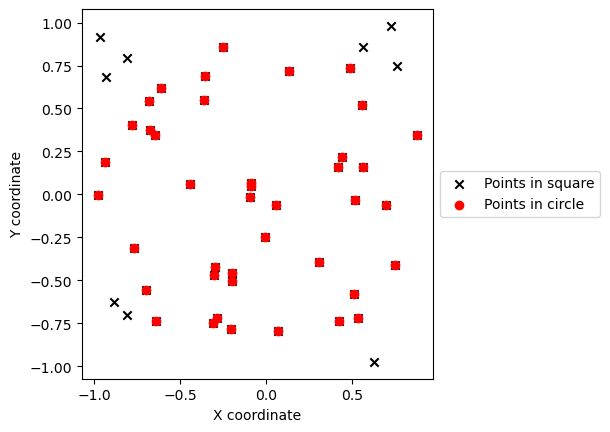
We now estimate \(\pi\) by using the length of the number points in the circle and in the quarter as approximation to their area.
# Let us estimate pi

pi_est = 4 * (len(in_circle) / len(in_square))

print('We estimate the value of pi to be: ' + str(pi_est) + '.')
We estimate the value of pi to be: 3.28.
Now with a few runs, we do not get a good answer.
In fact, a Monte Carlo approach needs more runs to converge.
You should explore how changing the number of runs changes your estimate of \(\pi\) (and how your calculation converges).
Using resampling for robust model inference (Level 2)#
2.1 Plate Motion - Geodetic Data#
For this tutorial, we use a GPS time series in the Pacific Northwest and explore the long term motions that are due to the Cascadia subduction zone.
We will download GPS time series from the University of Nevada - Reno data center.
# The station designation
sta="P395"

print("http://geodesy.unr.edu/gps_timeseries/tenv/IGS14/" + sta + ".tenv")
zip_file_url="http://geodesy.unr.edu/gps_timeseries/tenv/IGS14/"+ sta + ".tenv"
r = requests.get(zip_file_url)


# create a list of strings with itemized list above
ll = ['station ID (SSSS)','date (yymmmdd)',
'decimal year','modified Julian day','GPS week','day of GPS week',
'longitude (degrees) of reference meridian','delta e (m)',
'delta n (m)','delta v (m)','antenna height (m)',
'sigma e (m)','sigma n (m)','sigma v (m)',
'correlation en','correlation ev','correlation nv']


# transform r.content into a pandas dataframe
# first split r.content with \n separator
# Decode the content if it's in bytes
content_str = r.content.decode('utf-8')

# Split the content by the newline character
lines = content_str.split('\n')

# Now `lines` is a list of strings, each representing a line from the content
print(lines[0])

# then transform lines into a pandas dataframe
df = pd.DataFrame([x.split() for x in lines])
# assign column names to df a
df.columns = ll

#convert columns to numeric
df = df.apply(pd.to_numeric, errors='ignore')

df.dropna()
df.head()
http://geodesy.unr.edu/gps_timeseries/tenv/IGS14/P395.tenv
P395 06JAN25 2006.0671 53760 1359 3 -123.9 3347.67917 4987420.31375 53.03678 0.0083 0.00069 0.00105 0.00327 -0.04832 0.01695 -0.31816
| station ID (SSSS) | date (yymmmdd) | decimal year | modified Julian day | GPS week | day of GPS week | longitude (degrees) of reference meridian | delta e (m) | delta n (m) | delta v (m) | antenna height (m) | sigma e (m) | sigma n (m) | sigma v (m) | correlation en | correlation ev | correlation nv | |
|---|---|---|---|---|---|---|---|---|---|---|---|---|---|---|---|---|---|
| 0 | P395 | 06JAN25 | 2006.0671 | 53760.0 | 1359.0 | 3.0 | -123.9 | 3347.67917 | 4.987420e+06 | 53.03678 | 0.0083 | 0.00069 | 0.00105 | 0.00327 | -0.04832 | 0.01695 | -0.31816 |
| 1 | P395 | 06JAN26 | 2006.0698 | 53761.0 | 1359.0 | 4.0 | -123.9 | 3347.68086 | 4.987420e+06 | 53.03003 | 0.0083 | 0.00069 | 0.00104 | 0.00321 | -0.04648 | 0.00271 | -0.30970 |
| 2 | P395 | 06JAN27 | 2006.0726 | 53762.0 | 1359.0 | 5.0 | -123.9 | 3347.68072 | 4.987420e+06 | 53.03906 | 0.0083 | 0.00069 | 0.00105 | 0.00326 | -0.02367 | 0.00817 | -0.31941 |
| 3 | P395 | 06JAN28 | 2006.0753 | 53763.0 | 1359.0 | 6.0 | -123.9 | 3347.67938 | 4.987420e+06 | 53.04382 | 0.0083 | 0.00069 | 0.00105 | 0.00324 | -0.03681 | 0.00908 | -0.30515 |
| 4 | P395 | 06JAN29 | 2006.0780 | 53764.0 | 1360.0 | 0.0 | -123.9 | 3347.68042 | 4.987420e+06 | 53.03513 | 0.0083 | 0.00068 | 0.00105 | 0.00328 | -0.04815 | 0.00619 | -0.33029 |
# remove first value for delta e, delta n, delta v to make relative position with respect to the first time. Add these as new columns
df['new delta e (m)'] = df['delta e (m)'] - df['delta e (m)'].values[0]
df['new delta n (m)'] = df['delta n (m)'] - df['delta n (m)'].values[0]
df['new delta v (m)'] = df['delta v (m)'] - df['delta v (m)'].values[0]
df.head()
| station ID (SSSS) | date (yymmmdd) | decimal year | modified Julian day | GPS week | day of GPS week | longitude (degrees) of reference meridian | delta e (m) | delta n (m) | delta v (m) | antenna height (m) | sigma e (m) | sigma n (m) | sigma v (m) | correlation en | correlation ev | correlation nv | new delta e (m) | new delta n (m) | new delta v (m) | |
|---|---|---|---|---|---|---|---|---|---|---|---|---|---|---|---|---|---|---|---|---|
| 0 | P395 | 06JAN25 | 2006.0671 | 53760.0 | 1359.0 | 3.0 | -123.9 | 3347.67917 | 4.987420e+06 | 53.03678 | 0.0083 | 0.00069 | 0.00105 | 0.00327 | -0.04832 | 0.01695 | -0.31816 | 0.00000 | 0.00000 | 0.00000 |
| 1 | P395 | 06JAN26 | 2006.0698 | 53761.0 | 1359.0 | 4.0 | -123.9 | 3347.68086 | 4.987420e+06 | 53.03003 | 0.0083 | 0.00069 | 0.00104 | 0.00321 | -0.04648 | 0.00271 | -0.30970 | 0.00169 | -0.00067 | -0.00675 |
| 2 | P395 | 06JAN27 | 2006.0726 | 53762.0 | 1359.0 | 5.0 | -123.9 | 3347.68072 | 4.987420e+06 | 53.03906 | 0.0083 | 0.00069 | 0.00105 | 0.00326 | -0.02367 | 0.00817 | -0.31941 | 0.00155 | 0.00101 | 0.00228 |
| 3 | P395 | 06JAN28 | 2006.0753 | 53763.0 | 1359.0 | 6.0 | -123.9 | 3347.67938 | 4.987420e+06 | 53.04382 | 0.0083 | 0.00069 | 0.00105 | 0.00324 | -0.03681 | 0.00908 | -0.30515 | 0.00021 | -0.00150 | 0.00704 |
| 4 | P395 | 06JAN29 | 2006.0780 | 53764.0 | 1360.0 | 0.0 | -123.9 | 3347.68042 | 4.987420e+06 | 53.03513 | 0.0083 | 0.00068 | 0.00105 | 0.00328 | -0.04815 | 0.00619 | -0.33029 | 0.00125 | -0.00162 | -0.00165 |
plt.plot(df['decimal year'], df['new delta e (m)'], label='East displacement')
[<matplotlib.lines.Line2D at 0x7f9ce7df3250>]
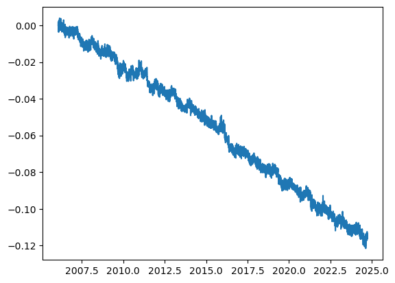
2.2 Linear regression#
There is a clean linear trend in the horizontal position data over the course of the past 16 years. We can fit the data using:
\(E(t) = V_e t + u_e,\)
\(N(t) = V_n t + u_n,\)
where \(t\) is time. We want to regress the data to find the coefficients \(V_e\), \(u_e\), \(V_n\), \(u_n\). The displacements are mostly westward, so we will just focus on the East \(E(t)\) component for this exercise. The coefficients \(u_e\) and \(u_n\) are the intercept at \(t=0\). They are not zero in this case because \(t\) starts in 2006. The coefficients \(V_e\) and \(V_n\) have the dimension of velocities:
\(V_e \sim E(t) / t\) , \(V_n \sim N(t) / t\) ,
therefore, we will use this example to discuss a simple linear regression and resampling method. We will use both a Scipy function and a Scikit-learn function.
To measure a fit performance, we will measure how well the variance is reduced by fitting the data (scatter points) against the model. The variance is:
\(\text{Var}(x) = 1/n \sum_{i=1}^n (x_i-\hat{x})^2\),
where \(\hat{x}\) is the mean of \(x\). When fitting the regression, we predict the values \(x_{pred}\). The residuals are the differences between the data and the predicted values: \(e = x - x_{pred} \). \(R^2\) or coefficient of determination is:
\(R^2 = 1 - \text{Var}(x-x_{pred}) /\text{Var}(x) = 1 - \text{Var}(e) /\text{Var}(x) \)
The smaller the error, the “better” the fit (we will discuss later that a fit can be too good!), the closer \(R^2\) is to one.
# remove nans with dropna for the specific delta e column and replace df with the new dataframe
df = df.dropna(subset=['delta e (m)'])
df.head()
| station ID (SSSS) | date (yymmmdd) | decimal year | modified Julian day | GPS week | day of GPS week | longitude (degrees) of reference meridian | delta e (m) | delta n (m) | delta v (m) | antenna height (m) | sigma e (m) | sigma n (m) | sigma v (m) | correlation en | correlation ev | correlation nv | new delta e (m) | new delta n (m) | new delta v (m) | |
|---|---|---|---|---|---|---|---|---|---|---|---|---|---|---|---|---|---|---|---|---|
| 0 | P395 | 06JAN25 | 2006.0671 | 53760.0 | 1359.0 | 3.0 | -123.9 | 3347.67917 | 4.987420e+06 | 53.03678 | 0.0083 | 0.00069 | 0.00105 | 0.00327 | -0.04832 | 0.01695 | -0.31816 | 0.00000 | 0.00000 | 0.00000 |
| 1 | P395 | 06JAN26 | 2006.0698 | 53761.0 | 1359.0 | 4.0 | -123.9 | 3347.68086 | 4.987420e+06 | 53.03003 | 0.0083 | 0.00069 | 0.00104 | 0.00321 | -0.04648 | 0.00271 | -0.30970 | 0.00169 | -0.00067 | -0.00675 |
| 2 | P395 | 06JAN27 | 2006.0726 | 53762.0 | 1359.0 | 5.0 | -123.9 | 3347.68072 | 4.987420e+06 | 53.03906 | 0.0083 | 0.00069 | 0.00105 | 0.00326 | -0.02367 | 0.00817 | -0.31941 | 0.00155 | 0.00101 | 0.00228 |
| 3 | P395 | 06JAN28 | 2006.0753 | 53763.0 | 1359.0 | 6.0 | -123.9 | 3347.67938 | 4.987420e+06 | 53.04382 | 0.0083 | 0.00069 | 0.00105 | 0.00324 | -0.03681 | 0.00908 | -0.30515 | 0.00021 | -0.00150 | 0.00704 |
| 4 | P395 | 06JAN29 | 2006.0780 | 53764.0 | 1360.0 | 0.0 | -123.9 | 3347.68042 | 4.987420e+06 | 53.03513 | 0.0083 | 0.00068 | 0.00105 | 0.00328 | -0.04815 | 0.00619 | -0.33029 | 0.00125 | -0.00162 | -0.00165 |
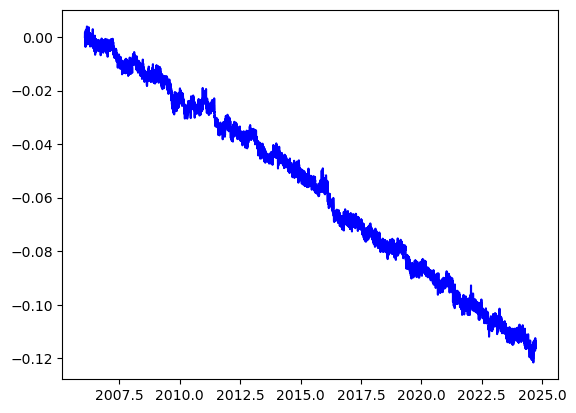
plt.plot(df['decimal year'], df['new delta e (m)'], label='East displacement')
[<matplotlib.lines.Line2D at 0x7f9ce790e2c0>]

df.head()
| station ID (SSSS) | date (yymmmdd) | decimal year | modified Julian day | GPS week | day of GPS week | longitude (degrees) of reference meridian | delta e (m) | delta n (m) | delta v (m) | antenna height (m) | sigma e (m) | sigma n (m) | sigma v (m) | correlation en | correlation ev | correlation nv | new delta e (m) | new delta n (m) | new delta v (m) | |
|---|---|---|---|---|---|---|---|---|---|---|---|---|---|---|---|---|---|---|---|---|
| 0 | P395 | 06JAN25 | 2006.0671 | 53760.0 | 1359.0 | 3.0 | -123.9 | 3347.67917 | 4.987420e+06 | 53.03678 | 0.0083 | 0.00069 | 0.00105 | 0.00327 | -0.04832 | 0.01695 | -0.31816 | 0.00000 | 0.00000 | 0.00000 |
| 1 | P395 | 06JAN26 | 2006.0698 | 53761.0 | 1359.0 | 4.0 | -123.9 | 3347.68086 | 4.987420e+06 | 53.03003 | 0.0083 | 0.00069 | 0.00104 | 0.00321 | -0.04648 | 0.00271 | -0.30970 | 0.00169 | -0.00067 | -0.00675 |
| 2 | P395 | 06JAN27 | 2006.0726 | 53762.0 | 1359.0 | 5.0 | -123.9 | 3347.68072 | 4.987420e+06 | 53.03906 | 0.0083 | 0.00069 | 0.00105 | 0.00326 | -0.02367 | 0.00817 | -0.31941 | 0.00155 | 0.00101 | 0.00228 |
| 3 | P395 | 06JAN28 | 2006.0753 | 53763.0 | 1359.0 | 6.0 | -123.9 | 3347.67938 | 4.987420e+06 | 53.04382 | 0.0083 | 0.00069 | 0.00105 | 0.00324 | -0.03681 | 0.00908 | -0.30515 | 0.00021 | -0.00150 | 0.00704 |
| 4 | P395 | 06JAN29 | 2006.0780 | 53764.0 | 1360.0 | 0.0 | -123.9 | 3347.68042 | 4.987420e+06 | 53.03513 | 0.0083 | 0.00068 | 0.00105 | 0.00328 | -0.04815 | 0.00619 | -0.33029 | 0.00125 | -0.00162 | -0.00165 |
# now let's find the trends and detrend the data.
from scipy import stats
# linear regression such that: displacement = Velocity * time
# velocity in the East component.

Ve, intercept, r_value, p_value, std_err = stats.linregress(df['decimal year'],df['new delta e (m)'])
# horizontal plate motion:
print(sta,"overall plate motion there",Ve,'m/year')
print("parameters: Coefficient of determination %f4.2, P-value %f4.2, standard deviation of errors %f4.2"\
      %(r_value,p_value,std_err))
P395 overall plate motion there -0.006439731291127395 m/year
parameters: Coefficient of determination -0.9970084.2, P-value 0.0000004.2, standard deviation of errors 0.0000064.2
np.isnan(df['new delta e (m)']).any()
False
We can also use the scikit-learn package:
from sklearn.linear_model import LinearRegression
# convert the data into numpy arrays.
E = np.asarray(df['new delta e (m)']).reshape(-1, 1)# reshaping was necessary to be an argument of Linear regress
# E = np.asarray(df['east'][df['station']==sta]).reshape(-1, 1)# reshaping was necessary to be an argument of Linear regress
# make a new time array
t = np.asarray(df['decimal year']).reshape(-1, 1)
tt = np.linspace(np.min(t),np.max(t),1000)

# perform the linear regression. First we will use the entire available data
regr = LinearRegression()
# we will first perform the fit:
regr.fit(t,E)
# We will first predict the fit:
Epred=regr.predict(t)

# The coefficients
print('Coefficient / Velocity eastward (mm/year): ', regr.coef_[0][0])
# plot the data
plt.plot(t,E,'b',label='data')
Coefficient / Velocity eastward (mm/year): -0.006439731291127396
[<matplotlib.lines.Line2D at 0x7f9cd8af7670>]
To evaluate the errors of the model fit using the module sklearn, we will use the following function
from sklearn.metrics import mean_squared_error, r2_score
# The mean squared error
print('Mean squared error (mm): %.2f'
      % mean_squared_error(E, Epred))
# The coefficient of determination: 1 is the perfect prediction
print('Coefficient of determination: %.2f'
      % r2_score(E, Epred))
Mean squared error (mm): 0.00
Coefficient of determination: 0.99
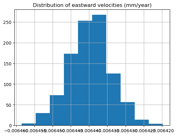
2.3 Bootstrapping#
Now we will use again bootstrapping to estimate the slope of the regression over many resampled data.
Scikit-learn seems to have deprecated the bootstrap function, but we can find resample in the utils module. Make sure you use replace=True.
For reproducible results, you can select a fixed random_state=int to be kept in the workflow. Usually bootstrapping is done over many times (unlike K-fold cross validation).
from sklearn.utils import resample
k=1000
vel = np.zeros(k) # initalize a vector to store the regression values
mse = np.zeros(k)
r2s = np.zeros(k)
i=0
for iik in range(k):
    ii = resample(np.arange(len(E)),replace=True,n_samples=len(E))# new indices
    E_b, t_b = E[ii], t[ii]
    # now fit the data on the training set.
    regr = LinearRegression()
    # Fit on training data:
    regr.fit(t_b,E_b)
    Epred_val=regr.predict(t) # test on the validation set.

    # The coefficients
    vel[i]= regr.coef_[0][0]
    i+=1

# the data shows clearly a trend, so the predictions of the trends are close to each other:
print("mean of the velocity estimates %f4.2 and the standard deviation %f4.2"%(np.mean(vel),np.std(vel)))

plt.hist(vel,10);plt.title('Distribution of eastward velocities (mm/year)');plt.grid(True)
# only show a few values in the x-axis

plt.show()
mean of the velocity estimates -0.0064404.2 and the standard deviation 0.0000064.2