3.1 Clustering
Contents
3.1 Clustering#
Clustering is a form of unsupervised classification because the goal is to discover structure on the basis of data features. Its primary objective is to unveil inherent structures within datasets based on their features. In essence, clustering endeavors to identify coherent subgroups among the observations.
The notion of homogeneity within a group is quantified through the concept of ‘distance’ between data points. This metric plays a pivotal role in the clustering process, aiding in the discernment of how similar or dissimilar data points are from one another.
This tutorial does not cover all possible clustering methods. No single clustering method works best for all scenario, it depends strongly on the inherent data struture. A simple summary, with toy examples of 2D data structure, is available in the sklearn package.
This lecture focuses on fundamental concepts that are relevant to the geosciences: 1) definition of distance and illustrate the most basics concepts using most popular clustering algorithm 2) K-means clustering and 3) agglomerative clustering.
1. Distance#
Understanding the concept of distance is crucial in machine learning, especially when it comes to clustering in the geosciences. Distance serves as a fundamental measure of dissimilarity or similarity between data points. Distance is also later used for calculating the loss and cost when training deep learning models.
There are various ways to estimate and quantify distance between data points. Some of the most commonly used distance metrics include:
Euclidean Distance: This is the straight-line distance between two data points in a multidimensional space. It is often used when the data features have similar units or scales. \(d(\mathbf{x},\mathbf{y}) = \sqrt{ \sum_{i=1}^N (x_i-y_i)^2 }/N\)
Manhattan Distance: Also known as the ‘L1’ distance, it measures the sum of the absolute differences between corresponding elements of two data points. It’s suitable when movement along axes is restricted, such as in grid-based data. \(d(\mathbf{x},\mathbf{y}) = \sum_{i=1}^N |x_i-y_i| /N\)
Geodesic Distance: Geodesic distance measures the shortest path between two points on the surface of a sphere, which is crucial for studying Earth’s geography, including GPS navigation and geodetic measurements.
Correlation-Based Distances: In geophysical and geospatial data analysis, correlation-based distance metrics like Pearson correlation or Spearman rank correlation are often used to assess relationships between variables.
Covariance-Based Distances: These distances, which take into account the spatial covariance or variogram models, are prevalent in geostatistics and spatial analysis.
Cosine Similarity: This metric calculates the cosine of the angle between two data vectors, providing a measure of their similarity, particularly in high-dimensional spaces. It’s frequently used for text or image data.
Scikit-learn contains the most commonly used metrics in the context of Classic ML under the package metrics.DistanceMetric. More details in this scikit-learn documentation.
Relation to PCA Clustering and PCA both simplify the data via a small number of summaries. But the differences are:
PCA seeks to reduce the dimensionality of the data, to find a low-dimensional representation of the data that explains a good fraction of the data variance,
Clustering seeks to find homogeneous groups within the observations.
In fact, it is common to combine both for complex and high dimensional data: 1) PCA, 2) clustering on the PCs.
There are two main methods using clustering, k-means clustering and hierarchical clustering.
The toolbox scikit-learn has a collection of clustering algorithms and detailed documentation with tutorials.
2. Tutorial set up#
Import useful Python packages
import matplotlib.pyplot as plt
import numpy as np
import pandas as pd
import random
import wget
# from math import cos, sin, pi, sqrt
# from mpl_toolkits.mplot3d import Axes3D
from sklearn import preprocessing
from sklearn.decomposition import PCA
import plotly.express as px
import os
Data#
We will use flow cytometer data.
The data file was provided by Katherine Qi from the UW SeaFlow group. The data is abundance and optical properties of phytoplankton The file has attributes about each particle, such as normalized scatter, red, orange, and green. These are measurements from the instrument itself from light scattering. Other parameters, like diam (diameter) and Qc (carbon quota) are estimated from the light scatter measurements.
# download data
cc=wget.download("https://www.dropbox.com/s/dwa82x6xhjkhyw8/ug3_FCM_distribution.feather?dl=1")
read the data
# this is some underway data collected from a cruise in 2019
os.replace("ug3_FCM_distribution.feather",'../../../ug3_FCM_distribution.feather')
underway_g3 = pd.read_feather("../../../ug3_FCM_distribution.feather")
print(underway_g3.columns)
underway_g3.head()
Index(['filename', 'pop', 'norm.scatter', 'norm.red', 'norm.orange',
       'norm.green', 'diam_lwr', 'Qc_lwr', 'diam_mid', 'Qc_mid', 'diam_upr',
       'Qc_upr', 'date', 'file', 'label', 'lat', 'lon', 'depth', 'replicate',
       'volume', 'stain', 'flag', 'comments'],
      dtype='object')
| filename | pop | norm.scatter | norm.red | norm.orange | norm.green | diam_lwr | Qc_lwr | diam_mid | Qc_mid | ... | file | label | lat | lon | depth | replicate | volume | stain | flag | comments | |
|---|---|---|---|---|---|---|---|---|---|---|---|---|---|---|---|---|---|---|---|---|---|
| 0 | towfish_001.fcs | prochloro | 0.009565 | 0.008967 | 0.001417 | 0.003938 | 0.540813 | 0.030637 | 0.653386 | 0.049902 | ... | towfish_001 | T20.28.05 | 30.0935 | -158.0003 | 5 | A | 173 | 0 | 2 | pro peak near low fluor noise |
| 1 | towfish_001.fcs | prochloro | 0.008924 | 0.015568 | 0.001417 | 0.003938 | 0.532844 | 0.029486 | 0.643588 | 0.047994 | ... | towfish_001 | T20.28.05 | 30.0935 | -158.0003 | 5 | A | 173 | 0 | 2 | pro peak near low fluor noise |
| 2 | towfish_001.fcs | prochloro | 0.005311 | 0.011982 | 0.001417 | 0.003938 | 0.478654 | 0.022358 | 0.577122 | 0.036229 | ... | towfish_001 | T20.28.05 | 30.0935 | -158.0003 | 5 | A | 173 | 0 | 2 | pro peak near low fluor noise |
| 3 | towfish_001.fcs | picoeuk | 0.925120 | 1.580796 | 0.003468 | 0.003938 | 1.548094 | 0.462018 | 2.003069 | 0.898166 | ... | towfish_001 | T20.28.05 | 30.0935 | -158.0003 | 5 | A | 173 | 0 | 2 | pro peak near low fluor noise |
| 4 | towfish_001.fcs | picoeuk | 0.277725 | 0.207073 | 0.001417 | 0.003938 | 1.136778 | 0.208269 | 1.416857 | 0.367623 | ... | towfish_001 | T20.28.05 | 30.0935 | -158.0003 | 5 | A | 173 | 0 | 2 | pro peak near low fluor noise |
5 rows × 23 columns
files = list(pd.unique(underway_g3['filename']))
print(files)
['towfish_001.fcs', 'towfish_002.fcs', 'towfish_003.fcs', 'towfish_004.fcs', 'towfish_005.fcs', 'towfish_006.fcs', 'towfish_007.fcs', 'towfish_008.fcs', 'towfish_009.fcs', 'towfish_010.fcs', 'towfish_011.fcs', 'towfish_012.fcs', 'towfish_013.fcs', 'towfish_014.fcs', 'towfish_015.fcs', 'towfish_016.fcs', 'towfish_017.fcs', 'towfish_018.fcs', 'towfish_019.fcs', 'towfish_020.fcs', 'underway_002.fcs', 'underway_003.fcs', 'underway_004.fcs', 'underway_005.fcs', 'underway_006.fcs', 'underway_007.fcs', 'underway_008.fcs', 'underway_009.fcs', 'underway_010.fcs', 'underway_011.fcs', 'underway_012.fcs', 'underway_013.fcs', 'underway_014.fcs', 'underway_015.fcs', 'underway_017.fcs', 'underway_018.fcs', 'underway_019.fcs', 'underway_020.fcs', 'underway_021.fcs', 'underway_022.fcs', 'underway_023.fcs', 'underway_024.fcs', 'underway_025.fcs', 'underway_026.fcs', 'underway_027.fcs', 'underway_028.fcs', 'underway_029.fcs', 'underway_030.fcs', 'underway_031.fcs', 'underway_032.fcs', 'underway_033.fcs', 'underway_034.fcs', 'underway_035.fcs', 'underway_036.fcs', 'underway_037.fcs', 'underway_038.fcs', 'underway_039.fcs', 'underway_040.fcs', 'underway_041.fcs', 'underway_042.fcs', 'underway_043.fcs', 'underway_044.fcs', 'underway_045.fcs', 'underway_046.fcs', 'underway_047.fcs', 'underway_048.fcs', 'underway_049.fcs', 'underway_050.fcs', 'underway_051.fcs', 'underway_052.fcs', 'underway_053.fcs', 'underway_054.fcs', 'underway_055.fcs', 'underway_056.fcs', 'underway_057.fcs', 'underway_058.fcs', 'underway_059.fcs', 'underway_060.fcs', 'underway_061.fcs', 'underway_062.fcs', 'underway_063.fcs', 'underway_064.fcs', 'underway_065.fcs', 'underway_066.fcs', 'underway_067.fcs', 'underway_068.fcs', 'underway_069.fcs', 'underway_070.fcs', 'underway_071.fcs', 'underway_072.fcs', 'underway_073.fcs', 'underway_074.fcs', 'underway_075.fcs', 'underway_076.fcs', 'underway_077.fcs', 'underway_078.fcs', 'underway_079.fcs', 'underway_080.fcs', 'underway_081.fcs', 'underway_082.fcs', 'underway_083.fcs', 'underway_084.fcs', 'underway_085.fcs', 'underway_086.fcs', 'underway_087.fcs', 'underway_088.fcs']
Each file is 1 sample taken at a certain time, location, and depth. There are also replicates, or even triplicates, run on the same spatiotemporal scale to get uncertainty estimations on the instrument. We can either ignore the replicates/triplicates or take the mean.
test1 = underway_g3[underway_g3['filename']==files[1]]
px.scatter(test1, 'norm.scatter', 'norm.red', color='pop',log_x=True, log_y=True)
px.scatter(test1, 'norm.scatter','norm.orange',color='pop',log_x=True,log_y=True)
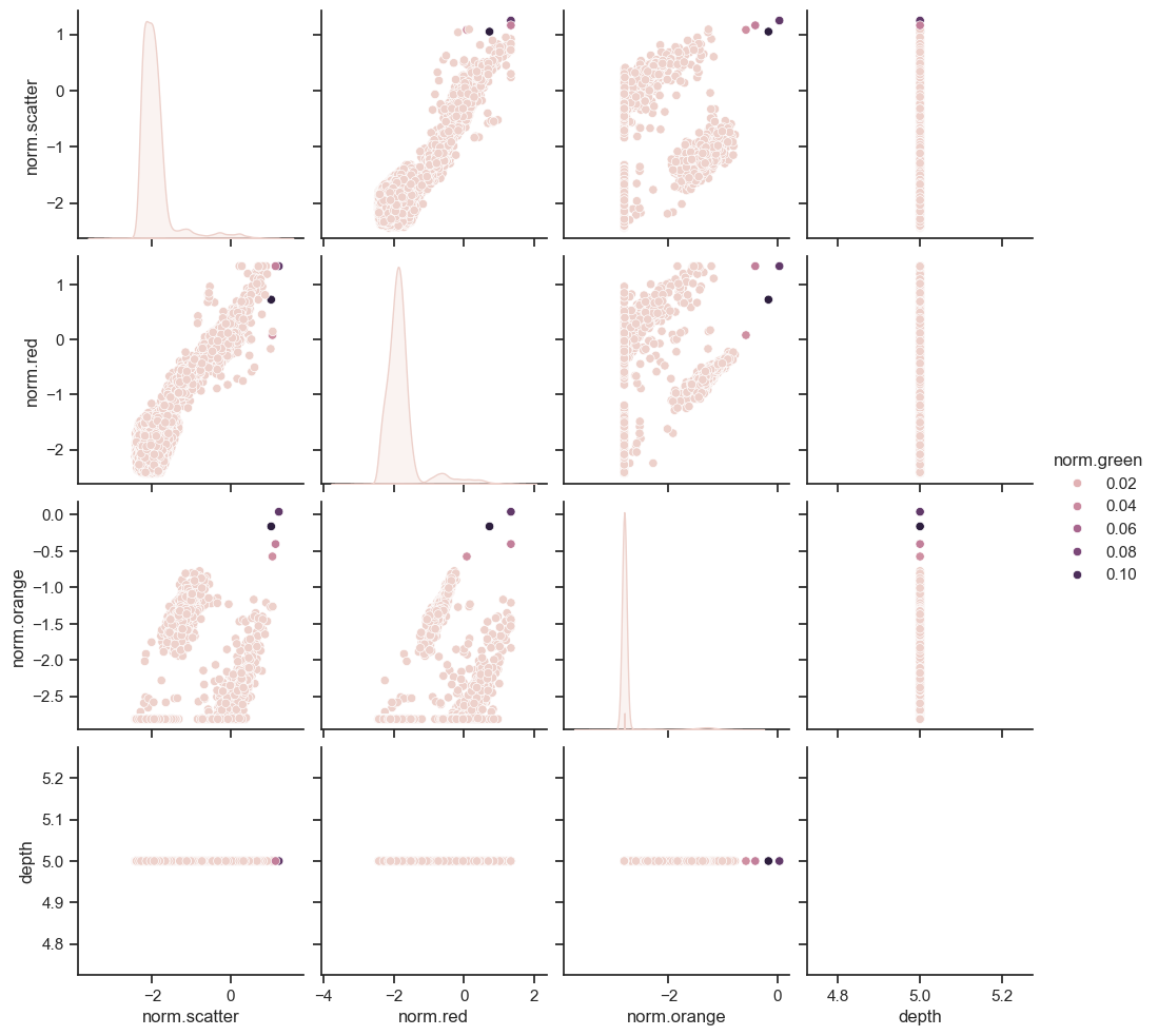
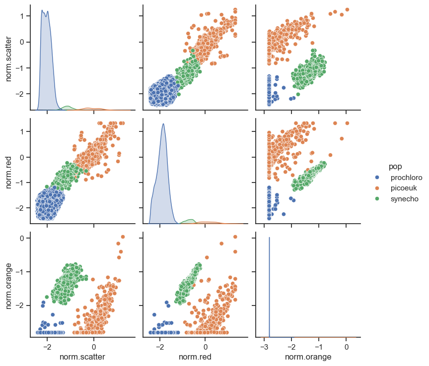
Typically, populations are gated based on their log-transformed normalized scatter (x) and red (y). Orange flourescence can be used in addition to gate the synecho population. We can see there are 3 populations here, and these were previously gated from the parameters above.
import seaborn as sns
sns.set_theme(style="ticks")
df = test1[['norm.scatter','norm.red','norm.orange','norm.green','depth']]
df['norm.scatter'] = np.log10(df['norm.scatter'])
df['norm.red'] = np.log10(df['norm.red'])
df['norm.orange'] = np.log10(df['norm.orange'])
sns.pairplot(df, hue="norm.green")
/var/folders/js/lzmy975n0l5bjbmr9db291m00000gn/T/ipykernel_60185/123783465.py:4: SettingWithCopyWarning:


A value is trying to be set on a copy of a slice from a DataFrame.
Try using .loc[row_indexer,col_indexer] = value instead

See the caveats in the documentation: https://pandas.pydata.org/pandas-docs/stable/user_guide/indexing.html#returning-a-view-versus-a-copy

/var/folders/js/lzmy975n0l5bjbmr9db291m00000gn/T/ipykernel_60185/123783465.py:5: SettingWithCopyWarning:


A value is trying to be set on a copy of a slice from a DataFrame.
Try using .loc[row_indexer,col_indexer] = value instead

See the caveats in the documentation: https://pandas.pydata.org/pandas-docs/stable/user_guide/indexing.html#returning-a-view-versus-a-copy

/var/folders/js/lzmy975n0l5bjbmr9db291m00000gn/T/ipykernel_60185/123783465.py:6: SettingWithCopyWarning:


A value is trying to be set on a copy of a slice from a DataFrame.
Try using .loc[row_indexer,col_indexer] = value instead

See the caveats in the documentation: https://pandas.pydata.org/pandas-docs/stable/user_guide/indexing.html#returning-a-view-versus-a-copy
<seaborn.axisgrid.PairGrid at 0x2b17a0f10>
sns.set_theme(style="ticks")
df = test1[['norm.scatter','norm.red','norm.orange','pop']]
df['norm.scatter'] = np.log10(df['norm.scatter'])
df['norm.red'] = np.log10(df['norm.red'])
df['norm.orange'] = np.log10(df['norm.orange'])
sns.pairplot(df, hue="pop")
/var/folders/js/lzmy975n0l5bjbmr9db291m00000gn/T/ipykernel_60185/3931145617.py:3: SettingWithCopyWarning:


A value is trying to be set on a copy of a slice from a DataFrame.
Try using .loc[row_indexer,col_indexer] = value instead

See the caveats in the documentation: https://pandas.pydata.org/pandas-docs/stable/user_guide/indexing.html#returning-a-view-versus-a-copy

/var/folders/js/lzmy975n0l5bjbmr9db291m00000gn/T/ipykernel_60185/3931145617.py:4: SettingWithCopyWarning:


A value is trying to be set on a copy of a slice from a DataFrame.
Try using .loc[row_indexer,col_indexer] = value instead

See the caveats in the documentation: https://pandas.pydata.org/pandas-docs/stable/user_guide/indexing.html#returning-a-view-versus-a-copy

/var/folders/js/lzmy975n0l5bjbmr9db291m00000gn/T/ipykernel_60185/3931145617.py:5: SettingWithCopyWarning:


A value is trying to be set on a copy of a slice from a DataFrame.
Try using .loc[row_indexer,col_indexer] = value instead

See the caveats in the documentation: https://pandas.pydata.org/pandas-docs/stable/user_guide/indexing.html#returning-a-view-versus-a-copy
<seaborn.axisgrid.PairGrid at 0x2b1edcd60>
3. K-means#
K-means is an unsupervised clustering method. The main idea is to separate the data into K distinct clusters. We then have two problems to solve. First, we need to find the k centroids of the k clusters. Then, we need to affect each data point to the cluster which centroid is the closest to the data point.
The goal is to partition \(n\) data points into \(k\) clusters. Each observation is labeled to a cluster with the nearest mean.
K-means is iterative:
assume initial values for the mean of each of the \(k\) clusters
Compute the distance for each observation to each of the \(k\) means
Label each observation as belonging to the nearest means
Find the center of mass (mean) of each group of labeled points. These are new means to step 1.
In the following, we denote \(n\) the number of data points, and \(p\) the number of features for each data point.
K-means only works with the Euclidian distance metrics. In fact, its core concept is to use the euclidian distance to measure and minimize inertia or within cluster variation.
n = len(df)
p = 3 #()
print('We have {:d} data points, and each one has {:d} features'.format(n, p))
We have 18470 data points, and each one has 3 features
Let’s define a numpy array with the 3 features and all of the data
data = np.zeros(shape=(n,p))
data[:,0] = df['norm.scatter']
data[:,1] = df['norm.red']
data[:,2] = df['norm.orange']
Let us define a function to initialize the centroid of the clusters. We choose random points within the range of values taken by the data.
def init_centers(data, k):
    """
    """
    # Initialize centroids
    centers = np.zeros((k, np.shape(data)[1]))
    # Loop on k centers
    for i in range(0, k):
        # Generate p random values between 0 and 1
        dist = np.random.uniform(size=np.shape(data)[1])
        # Use the random values to generate a point within the range of values taken by the data
        centers[i, :] = np.min(data, axis=0) + (np.max(data, axis=0) - np.min(data, axis=0)) * dist
    return centers
To be able to affect each data point to the closest centroid, we need to define the distance between two data points. The most common distance is the Euclidean distance:
\(d(x,y) = \sqrt{\sum_{i = 1}^p (x_i - y_i)^2}\)
where \(x\) and \(y\) are two data observation points with \(p\) variables.
We then define a function to compute the distance between each data point and each centroid.
def compute_distance(data, centers, k):
    """
    """
    # Initialize distance
    distance = np.zeros((np.shape(data)[0], k))
    # Loop on n data points
    for i in range(0, np.shape(data)[0]):
        # Loop on k centroids
        for j in range(0, k):
            # Compute distance
            distance[i, j] = sqrt(np.sum(np.square(data[i, :] - centers[j, :])))
    return distance
We now define a function to affect each data point to the cluster which centroid is the closest to the point. We also define an objective function that will be minimized until we reach convergence.
Our objective is to minimize the sum of the square of the distance between each point and the closest centroid:
\(obj = \sum_{j = 1}^k \sum_{i = 1}^{N_j} d(x^{(i)} , x^{(j)}) ^2\)
where \(x^{(i)}\) is the \(i^{th}\) point in the cluster \(j\), \(x^{(j)}\) is the centroid of the cluster \(j\), and \(N_j\) is the number of points in the cluster \(j\).
def compute_objective(distance, clusters):
    """
    """
    # Initialize objective
    objective = 0.0
    # Loop on n data points
    for i in range(0, np.shape(distance)[0]):
        # Add distance to the closest centroid
        objective = objective + distance[i, int(clusters[i])] ** 2.0
    return objective
def compute_clusters(distance):
    """
    """
    # Initialize clusters
    clusters = np.zeros(np.shape(distance)[0])
    # Loop on n data points
    for i in range(0, np.shape(distance)[0]):
        # Find closest centroid
        best = np.argmin(distance[i, :])
        # Assign data point to corresponding cluster
        clusters[i] = best
    return clusters
After all points are assigned to a cluster, compute the new location of the centroid. It is just the value of the mean of all the points affected to that cluster:
For \(1 \leq j \leq k\), \(x_p^{(j)} = \frac{1}{N_j} \sum_{i = 1}^{N_j} x_p^{(i)}\)
def compute_centers(data, clusters, k):
    """
    """
    # Initialize centroids
    centers = np.zeros((k, np.shape(data)[1]))
    # Loop on clusters
    for i in range(0, k):
        # Select all data points in this cluster
        subdata = data[clusters == i, :]
        # If no data point in this cluster, generate randomly a new centroid
        if (np.shape(subdata)[0] == 0):
            centers[i, :] = init_centers(data, 1)
        else:
            # Compute the mean location of all data points in this cluster
            centers[i, :] = np.mean(subdata, axis=0)
    return centers
We can now code the K-means algorithm by assembling all these functions. We stop the computation when the objective function no longer decreases.
def my_kmeans(data, k):
    """
    """
    # Initialize centroids
    centers = init_centers(data, k)
    # Initialize objective function to square of the maximum distance between two data points times number of data points
    objective_old = np.shape(data)[0] * np.sum(np.square(np.max(data, axis=0) - np.min(data, axis=0)))
    # Initialize clusters
    clusters_old = np.zeros(np.shape(data)[0])
    # Start loop until convergence
    stop_alg = False
    while stop_alg == False:
        # Compute distance between data points and centroids
        distance = compute_distance(data, centers, k)
        # Get new clusters
        clusters_new = compute_clusters(distance)
        # get new value of objective function
        objective_new = compute_objective(distance, clusters_new)
        # If objective function stops decreasing, end loop
        if objective_new >= objective_old:
            return (clusters_old, objective_old, centers)
        else:
            # Update the locations of the centroids
            centers = compute_centers(data, clusters_new, k)
            objective_old = objective_new
            clusters_old = clusters_new
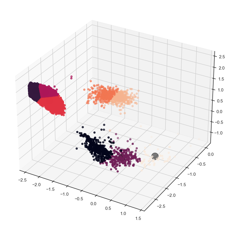
Run K-means with 4 clusters
k = 4
(clusters, objective, centers) = my_kmeans(data, k)
df["clusterID"]=clusters.astype('str')
fig = px.scatter_3d(df, x='norm.scatter', y='norm.red', z='norm.orange',
              color='clusterID')
fig.show()
# fig = plt.figure(figsize=(10, 10))
# ax = fig.add_subplot(111, projection='3d')
# ax.scatter(data[:, 1], data[:, 0], -data[:, 2], c=clusters)
# ax.scatter(centers[:, 1], centers[:, 0], -centers[:, 2], marker='o', s=300, c='black')
# ax.set_xlabel('norm.scatterer')
# ax.set_ylabel('norm.red')
# ax.set_ylabel('norm.orange')
# plt.title('Clusters for cytometer data')
/var/folders/js/lzmy975n0l5bjbmr9db291m00000gn/T/ipykernel_60185/1190913055.py:3: SettingWithCopyWarning:


A value is trying to be set on a copy of a slice from a DataFrame.
Try using .loc[row_indexer,col_indexer] = value instead

See the caveats in the documentation: https://pandas.pydata.org/pandas-docs/stable/user_guide/indexing.html#returning-a-view-versus-a-copy
K-means with Scikit learn#
We will now use scikit learn toolbox to run kmeans. Follow that tutorial and apply it to your problem.
from sklearn.cluster import KMeans

X = data
Y = np.asarray(df['pop'])

kmeans = KMeans(n_clusters=2, random_state=0).fit(data)
kmeans.labels_
/Users/marinedenolle/opt/miniconda3/envs/mlgeo/lib/python3.9/site-packages/sklearn/cluster/_kmeans.py:1416: FutureWarning:

The default value of `n_init` will change from 10 to 'auto' in 1.4. Set the value of `n_init` explicitly to suppress the warning
array([0, 0, 0, ..., 0, 0, 0], dtype=int32)
# explore different pipeline


estimators = [
    ("k_means_cyto_8", KMeans(n_clusters=8)),
    ("k_means_cyto_3", KMeans(n_clusters=3)),
    ("k_means_cyto_bad_init", KMeans(n_clusters=3, n_init=1, init="random")),
]

name,est=estimators[0]
est.fit(data)
labels = est.labels_

fig = plt.figure(0, figsize=(4, 3))

df["clusterID"]=labels.astype('str')
fig = px.scatter_3d(df, x='norm.scatter', y='norm.red', z='norm.orange',
              color='clusterID')
fig.show()
/Users/marinedenolle/opt/miniconda3/envs/mlgeo/lib/python3.9/site-packages/sklearn/cluster/_kmeans.py:1416: FutureWarning:

The default value of `n_init` will change from 10 to 'auto' in 1.4. Set the value of `n_init` explicitly to suppress the warning

/var/folders/js/lzmy975n0l5bjbmr9db291m00000gn/T/ipykernel_60185/3068295825.py:16: SettingWithCopyWarning:


A value is trying to be set on a copy of a slice from a DataFrame.
Try using .loc[row_indexer,col_indexer] = value instead

See the caveats in the documentation: https://pandas.pydata.org/pandas-docs/stable/user_guide/indexing.html#returning-a-view-versus-a-copy
<Figure size 400x300 with 0 Axes>
Practical tips for k-means#
How to evaluate the success of the clustering? How well separated are the clusters? There exist many ways to evaluate the quality of the clusters. Scikit-learn has summarized and packaged these tools into the module
sklearn.metrics. See documentation here. Usually, high scores are better. Here is a summary:If the data has ground-truth labels (e.g., population of the cyto data), we can use several metrics:
homogeneity (each cluster contains only members of a given class,
metrics.homgeneity_score(clusterID,true_label)), completeness (all members of a given class are assigned the same cluster,metrics.completeness_score), V-measure (2 x homogeneity x completeness / (homogeneity+completeness),metrics.v_measure_score) and all threemetrics.homogeneity_completeness_v_measure(clusterID,true_label).Fowlkes-Mallows index, FMI, that uses TP (True Positive), FP (False Positive), FN (False Negative). Is 0.0 for random cluster assignment and 1.0 for perfect label assignments.
If the data does not have ground truth label, you can use:
silhouette coefficient using the module
metrics.silhouette_score), a high score or coefficient is better. It quantifies how tight the data within the clusters are and how well separated the clusters are. More details on implementation and visualization of the silhouette score here.
The number of clusters \(k\) is a tunable parameter. To find the optimal number of clusters, we discuss below a few strategies.
The optimization of k-means may have local minima. The result therefore may different due to the initialiation of the clusters. It is recommended to use:
repeat random initialization, repeat k-means, and use the best set of cluster (one that has the lowest final error)
choose K-means++ initialization scheme using the sklearn parameter
init='k-means++'. The algorithm selects initial cluster centroids using sampling based on an empirical probability distribution of the points’ contribution to the overall inertia.
The data variance of some of the features may affect the results. It may be difficult to find clusters if some of the data features (axis) are much larger than other. The data may need to be pre-processed (centered and scaled) or pre-conditions (e.g., PCA).
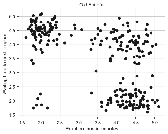
In the following, we take the example of a simple data sets. The Old Faithful is a geyser in Yellowstone. The data shows the time of the geyser eruption against the waiting time for the next eruptions.
faithful = pd.read_csv('faithful.csv')
data_faithful = faithful.to_numpy()
plt.plot(faithful.current, faithful.next, 'ko')
plt.xlabel('Eruption time in minutes')
plt.ylabel('Waiting time to next eruption')
plt.grid(True)
plt.title('Old Faithful')
Text(0.5, 1.0, 'Old Faithful')
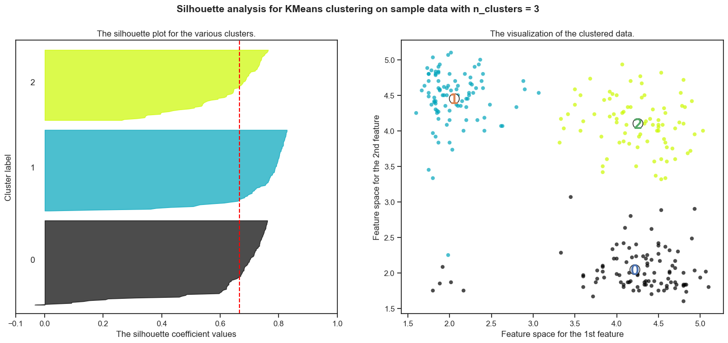
Silhouette analysis
The silhouette coefficient and silhouette score are metrics used to assess the quality of clustering in unsupervised learning.
Silhouette Coefficient: The silhouette coefficient for a data sample measures how similar it is to its own cluster (cohesion) compared to other clusters (separation). It is calculated for each data sample and ranges from -1 to 1. A high silhouette coefficient indicates that the object is well matched to its own cluster and poorly matched to neighboring clusters. Conversely, a low silhouette coefficient suggests that the object may be in the wrong cluster.
The formula for the silhouette coefficient (s) for a single data point is given by:
\( s(i) = \frac{b(i) - a(i)}{\max\{a(i), b(i)\}} \) where:
\(a(i)\) is the average distance from the \(i\)-th data point to the other data points in the same cluster.
\(b(i)\) is the smallest average distance from the \(i\)-th data point to data points in a different cluster, minimized over clusters.
Silhouette Score: The silhouette score is the average silhouette coefficient across all data samples in the dataset. It provides a global measure of how well-separated clusters are. The silhouette score ranges from -1 to 1 as well, where a high score indicates good clustering and a low score suggests overlapping or misclassified clusters.
The formula for the silhouette score is given by:
\( S = \frac{\sum_{i=1}^{N} s(i)}{N} \) where:
\(N\) is the number of data points in the dataset.
Interpretation:
A silhouette coefficient close to 1 indicates that the data point is well-matched to its own cluster and poorly matched to neighboring clusters, signifying a robust and distinct cluster.
A silhouette coefficient close to -1 suggests that the data point is possibly misclassified, as it is better matched to a neighboring cluster.
A silhouette coefficient around 0 indicates overlapping clusters.
For the silhouette score:
A score close to 1 implies well-defined clusters.
A score around 0 suggests overlapping clusters.
A negative score indicates that the majority of data points may be assigned to the wrong clusters.
In summary, silhouette analysis helps in selecting the optimal number of clusters and assessing the overall quality of clustering in unsupervised learning, providing valuable insights into the structure of the data.
# example of the silhouette score for the Old Faithful data
from sklearn.cluster import KMeans
from sklearn import metrics
from sklearn.metrics import silhouette_score, silhouette_samples

ncluster=3

kmeans_model = KMeans(n_clusters=ncluster, random_state=1).fit(data_faithful)
labels = kmeans_model.labels_
sc=silhouette_score(data_faithful, labels, metric='euclidean')
/Users/marinedenolle/opt/miniconda3/envs/mlgeo/lib/python3.9/site-packages/sklearn/cluster/_kmeans.py:1416: FutureWarning:

The default value of `n_init` will change from 10 to 'auto' in 1.4. Set the value of `n_init` explicitly to suppress the warning
import matplotlib.cm as cm
fig, (ax1, ax2) = plt.subplots(1, 2)
fig.set_size_inches(18, 7)
#The 1st subplot is the silhouette plot
# The silhouette coefficient can range from -1, 1 but in this example all
# lie within [-0.1, 1]
ax1.set_xlim([-0.1, 1])
# The (n_clusters+1)*10 is for inserting blank space between silhouette
# plots of individual clusters, to demarcate them clearly.
ax1.set_ylim([0, len(data_faithful) + (ncluster + 1) * 10])

# Initialize the clusterer with n_clusters value and a random generator
# seed of 10 for reproducibility.
clusterer = KMeans(n_clusters=ncluster, random_state=10)
cluster_labels = clusterer.fit_predict(data_faithful)

# The silhouette_score gives the average value for all the samples.
# This gives a perspective into the density and separation of the formed
# clusters
silhouette_avg = silhouette_score(data_faithful, cluster_labels)
print(
    "For n_clusters =",
    ncluster,
    "The average silhouette_score is :",
    silhouette_avg,
)

# Compute the silhouette scores for each sample
sample_silhouette_values = silhouette_samples(data_faithful, cluster_labels)

y_lower = 10
for i in range(ncluster):
    # Aggregate the silhouette scores for samples belonging to
    # cluster i, and sort them
    ith_cluster_silhouette_values = sample_silhouette_values[cluster_labels == i]

    ith_cluster_silhouette_values.sort()

    size_cluster_i = ith_cluster_silhouette_values.shape[0]
    y_upper = y_lower + size_cluster_i

    color = cm.nipy_spectral(float(i) / ncluster)
    ax1.fill_betweenx(
        np.arange(y_lower, y_upper),
        0,
        ith_cluster_silhouette_values,
        facecolor=color,
        edgecolor=color,
        alpha=0.7,
    )

    # Label the silhouette plots with their cluster numbers at the middle
    ax1.text(-0.05, y_lower + 0.5 * size_cluster_i, str(i))

    # Compute the new y_lower for next plot
    y_lower = y_upper + 10  # 10 for the 0 samples

ax1.set_title("The silhouette plot for the various clusters.")
ax1.set_xlabel("The silhouette coefficient values")
ax1.set_ylabel("Cluster label")

# The vertical line for average silhouette score of all the values
ax1.axvline(x=silhouette_avg, color="red", linestyle="--")

ax1.set_yticks([])  # Clear the yaxis labels / ticks
ax1.set_xticks([-0.1, 0, 0.2, 0.4, 0.6, 0.8, 1])

# 2nd Plot showing the actual clusters formed
colors = cm.nipy_spectral(cluster_labels.astype(float) / ncluster)
ax2.scatter(
    data_faithful[:, 0], data_faithful[:, 1], marker="o", s=30, lw=0, alpha=0.7, c=colors, edgecolor="k"
)

# Labeling the clusters
centers = clusterer.cluster_centers_
# Draw white circles at cluster centers
ax2.scatter(
    centers[:, 0],
    centers[:, 1],
    marker="o",
    c="white",
    alpha=1,
    s=200,
    edgecolor="k",
)

for i, c in enumerate(centers):
    ax2.scatter(c[0], c[1], marker="$%d$" % i, alpha=1, s=200, edgecolor=None)

ax2.set_title("The visualization of the clustered data.")
ax2.set_xlabel("Feature space for the 1st feature")
ax2.set_ylabel("Feature space for the 2nd feature")

plt.suptitle(
    "Silhouette analysis for KMeans clustering on sample data with n_clusters = %d"
    % ncluster,
    fontsize=14,
    fontweight="bold",
)
For n_clusters = 3 The average silhouette_score is : 0.6660137226595727
/Users/marinedenolle/opt/miniconda3/envs/mlgeo/lib/python3.9/site-packages/sklearn/cluster/_kmeans.py:1416: FutureWarning:

The default value of `n_init` will change from 10 to 'auto' in 1.4. Set the value of `n_init` explicitly to suppress the warning
Text(0.5, 0.98, 'Silhouette analysis for KMeans clustering on sample data with n_clusters = 3')
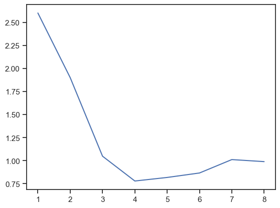
3. Choice of number of clusters: The Elbow Method#
The elbow method is designed to find the optimal number of clusters. It consists in performing the clustering algorithm with an increasing number of clusters \(k\) and select and measuring the average distance between data points and the cluster centroids. There are two typical metrics in the Elbow method
Distortion: It is calculated as the average of the squared distances from the cluster centers of the respective clusters. Typically, the Euclidean distance metric is used.
Inertia: It is the sum of squared distances of samples to their closest cluster center.
For each value of \(k\), we compute the mean of the square of the distance between the data points and the centroid of the cluster to which they belong. We then plot this value as a function of \(k\). Hopefully, it decreases and then reaches a plateau. The optimal number of clusters is the value for which it attains the minimum.
Let us use a different dataset to illustrate the elbow method.
def compute_elbow(data, clusters, centers, k):
    """
    """
    E = 0
    for i in range(0, k):
        distance = compute_distance(data[clusters == i, :], centers[i, :].reshape(1, -1), 1)
        E = E + np.mean(np.square(distance))
    return E
Compute the value of E for different values of the number of clusters
E = np.zeros(8)
for k in range(1, 9):
    (clusters, objective, centers) = my_kmeans(data_faithful, k)
    E[k - 1] = compute_elbow(data_faithful, clusters, centers, k)
Plot \(E\) as a function of \(k\) and see where reaches a minimum.
plt.plot(np.arange(1, 9), E)
[<matplotlib.lines.Line2D at 0x2ba38ac10>]
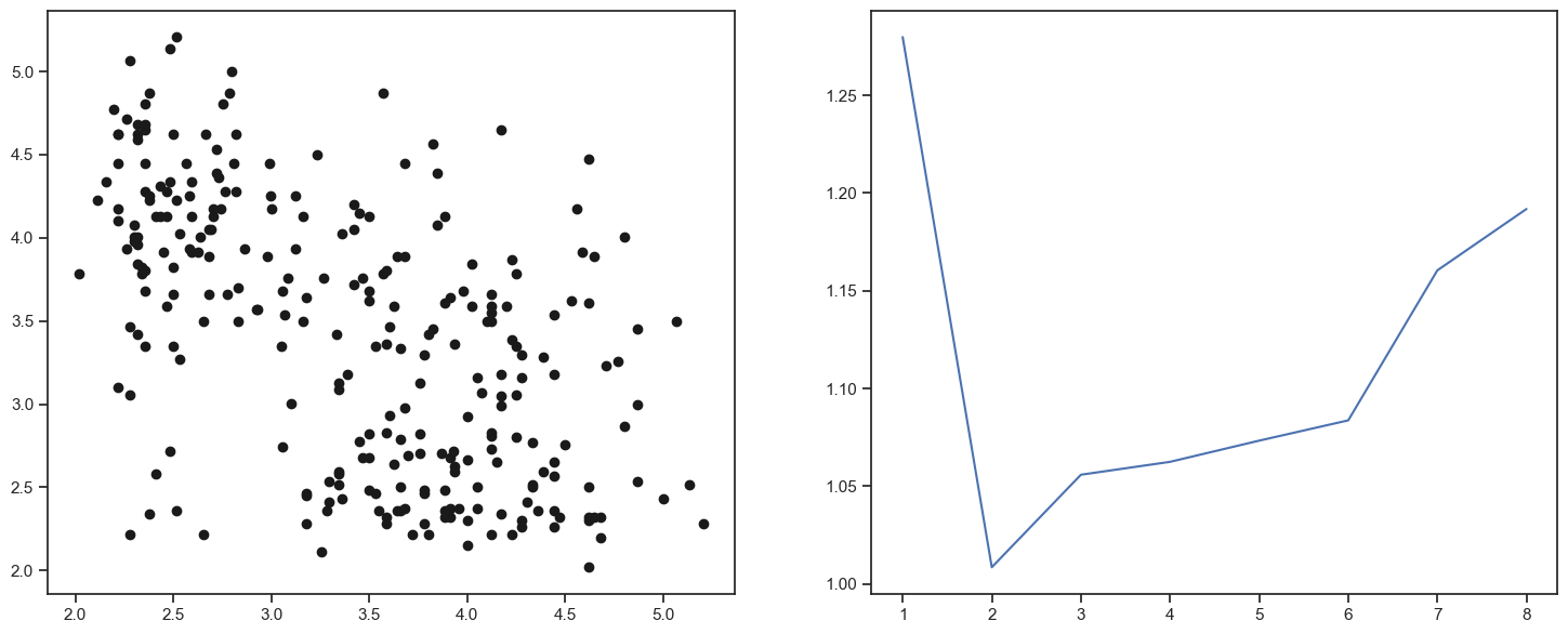
The elbow method does not always work very well. For example, see what happens when the points get closer to each other.
fig, (ax1, ax2) = plt.subplots(1, 2)
fig.set_size_inches(18, 7)
alpha = 0.5
origin = np.array([3, 3])
data_shrink = origin + alpha * np.sign(data_faithful - origin) * np.power(np.abs(data_faithful - origin), 2.0)
ax1.plot(data_shrink[:, 0], data_shrink[:, 1], 'ko')

E = np.zeros(8)
for k in range(1, 9):
    (clusters, objective, centers) = my_kmeans(data_shrink, k)
    E[k - 1] = compute_elbow(data_shrink, clusters, centers, k)
ax2.plot(np.arange(1, 9), E)
[<matplotlib.lines.Line2D at 0x2ba44ab50>]
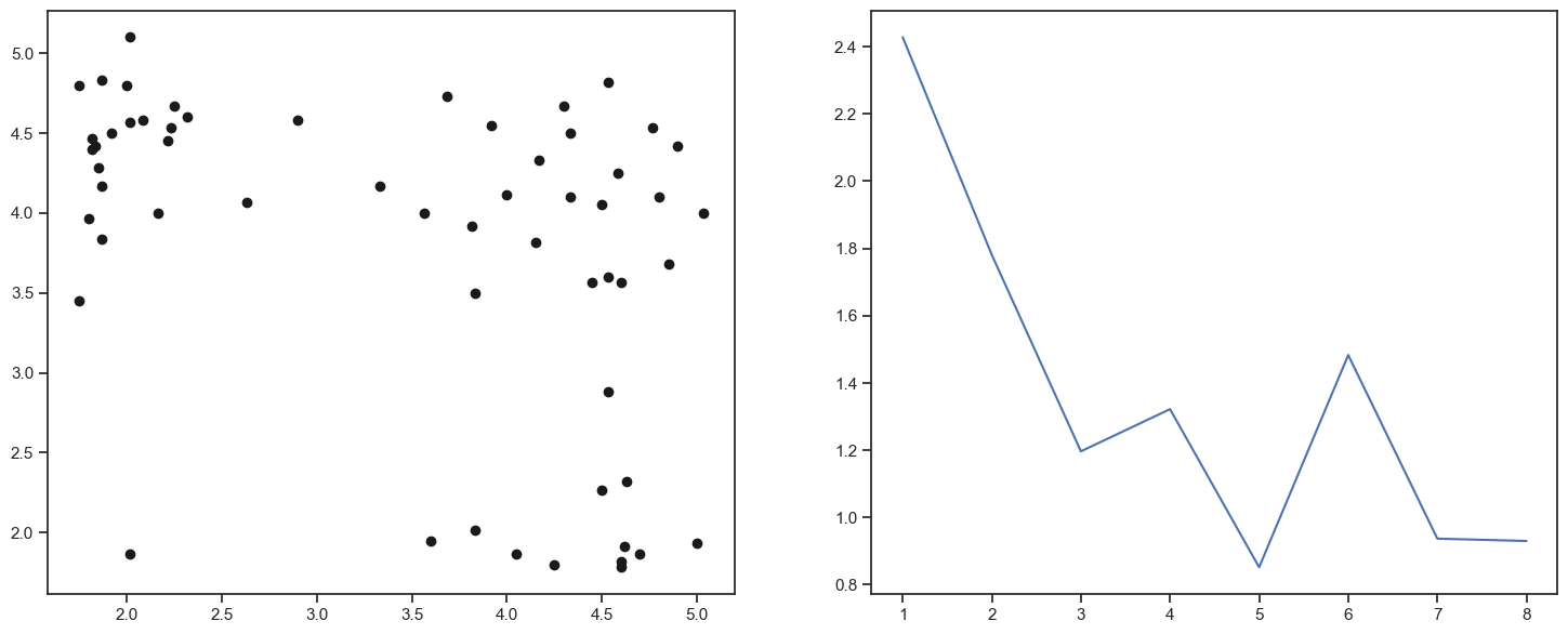
Let us see what happens when we decrease the number of data
fig, (ax1, ax2) = plt.subplots(1, 2)
fig.set_size_inches(18, 7)
alpha = 0.2
indices = np.random.uniform(size=np.shape(data_faithful)[0])
subdata = data_faithful[indices < alpha, :]
ax1.plot(subdata[:, 0], subdata[:, 1], 'ko')
E = np.zeros(8)
for k in range(1, 9):
    (clusters, objective, centers) = my_kmeans(subdata, k)
    E[k - 1] = compute_elbow(subdata, clusters, centers, k)
ax2.plot(np.arange(1, 9), E)
[<matplotlib.lines.Line2D at 0x2ba534b80>]
3. Repeat K-means#
Result is very sensitive to the location of the initial centroid. Repeat the clustering N times and choose the clustering with the best objective function
def repeat_kmeans(data, k, N):
    """
    """
    # Initialization
    objective = np.zeros(N)
    clusters = np.zeros((N, np.shape(data)[0]))
    centers = np.zeros((N, k, np.shape(data)[1]))
    # Run K-means N times
    for i in range(0, N):
        result = my_kmeans(data, k)
        clusters[i, :] = result[0]
        objective[i] = result[1]
        centers[i, :, :] = result[2]
        print(i/N*100)
    # Choose the clustering with the best value of the objective function
    best = np.argmin(objective)
    return (clusters[best, :], objective[best], centers[best, :, :])
Repeat k-means 50 times
N = 30
(clusters, objective, centers) = repeat_kmeans(data, k, N)
fig = plt.figure(figsize=(10, 10))
ax = fig.add_subplot(111, projection='3d')
ax.scatter(data[:, 1], data[:, 2], -data[:, 0], c=clusters)
ax.scatter(centers[:, 1], centers[:, 2], -centers[:, 0], marker='o', s=300, c='black')
0.0
3.3333333333333335
6.666666666666667
10.0
13.333333333333334
16.666666666666664
20.0
23.333333333333332
26.666666666666668
30.0
33.33333333333333
36.666666666666664
40.0
43.333333333333336
46.666666666666664
50.0
53.333333333333336
56.666666666666664
60.0
63.33333333333333
66.66666666666666
70.0
73.33333333333333
76.66666666666667
80.0
83.33333333333334
86.66666666666667
90.0
93.33333333333333
96.66666666666667
<mpl_toolkits.mplot3d.art3d.Path3DCollection at 0x2ba5f8bb0>
K-means can be a slow process to calculate and there are avenues to speed this up. One solution is to do mini-batch K-means, which takes a subset of data at each iteration to construct the centroids.
4. Hierarchical Clustering#
In K-means, we use the euclidian distance and prescribe the number of clusters K.
In hierarchical clustering, we choose difference distance metrics, visualize the data structure, and then decide on the number of clusters. There are two approaches to building the hierarchy of clusters:
Agglomerative: each point starts in each unique cluster. data is merged in pairs as on creates a hierarchy of clusters.
Divisive: initially, all data is into 1 cluster. The data is recursively split into smaller and smaller clusters.
There are several types of linkages. sklearn has detailed documentation, mostly for agglomerative: The different linkages methods are:
Ward minimizes the sum of squared differences within all clusters. It is a variance-minimizing approach and in this sense is similar to the k-means objective function but tackled with an agglomerative hierarchical approach.
Maximum or complete linkage minimizes the maximum distance between observations of pairs of clusters.
Average linkage minimizes the average of the distances between all observations of pairs of clusters.
Single linkage minimizes the distance between the closest observations of pairs of clusters.
We first import relevant packages
import numpy as np
import matplotlib.pyplot as plt
from matplotlib import rcParams
from scipy.cluster import hierarchy  #
from scipy.spatial.distance import pdist

rcParams.update({'font.size': 18})
plt.rcParams['figure.figsize'] = [12, 12]
Here, we create a fake data sets that has 2 clusters that intermingle in a few data points.
# Training and testing set sizes
n = 100 # Train

# Random ellipse 1 centered at (0,0)
x = np.random.randn(n)
y = 0.5*np.random.randn(n)

# Random ellipse 2 centered at (1,-2)
x2 = np.random.randn(n) + 1
y2 = 0.2*np.random.randn(n) - 2

# Rotate ellipse 2 by theta
theta = np.pi/4
A = np.zeros((2,2))
A[0,0] = np.cos(theta)
A[0,1] = -np.sin(theta)
A[1,0] = np.sin(theta)
A[1,1] = np.cos(theta)

x3 = A[0,0]*x2 + A[0,1]*y2
y3 = A[1,0]*x2 + A[1,1]*y2
plt.figure()
plt.plot(x[:],y[:],'ro')
plt.plot(x3[:],y3[:],'bo')
plt.show()
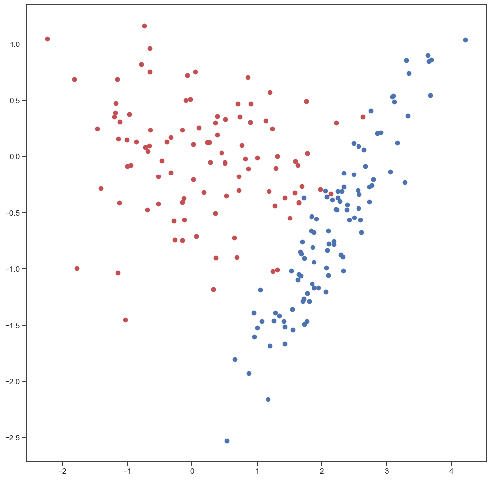
Combine these two data sets as one.
X1 = np.column_stack((x3[:],y3[:]))
X2 = np.column_stack((x[:],y[:]))
X = np.concatenate((X1,X2))
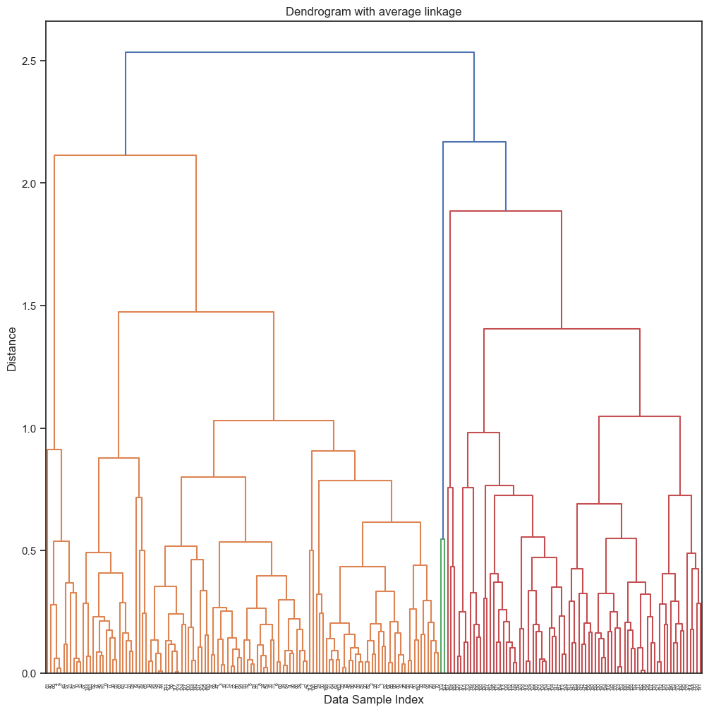
First we explore the dendograms
## Dendrograms
Y = pdist(X,metric='euclidean')
Z = hierarchy.linkage(Y,method='average')
thresh = 0.85*np.max(Z[:,2])

plt.figure()
dn = hierarchy.dendrogram(Z,p=100,color_threshold=thresh)
plt.xlabel('Data Sample Index')
plt.ylabel('Distance')
plt.title('Dendrogram with average linkage')
plt.show()
thresh = 0.25*np.max(Z[:,2])
plt.figure()
dn = hierarchy.dendrogram(Z,p=100,color_threshold=thresh)
plt.xlabel('Data Sample Index')
plt.ylabel('Distance')
plt.title('Dendrogram with average linkage')
plt.show()
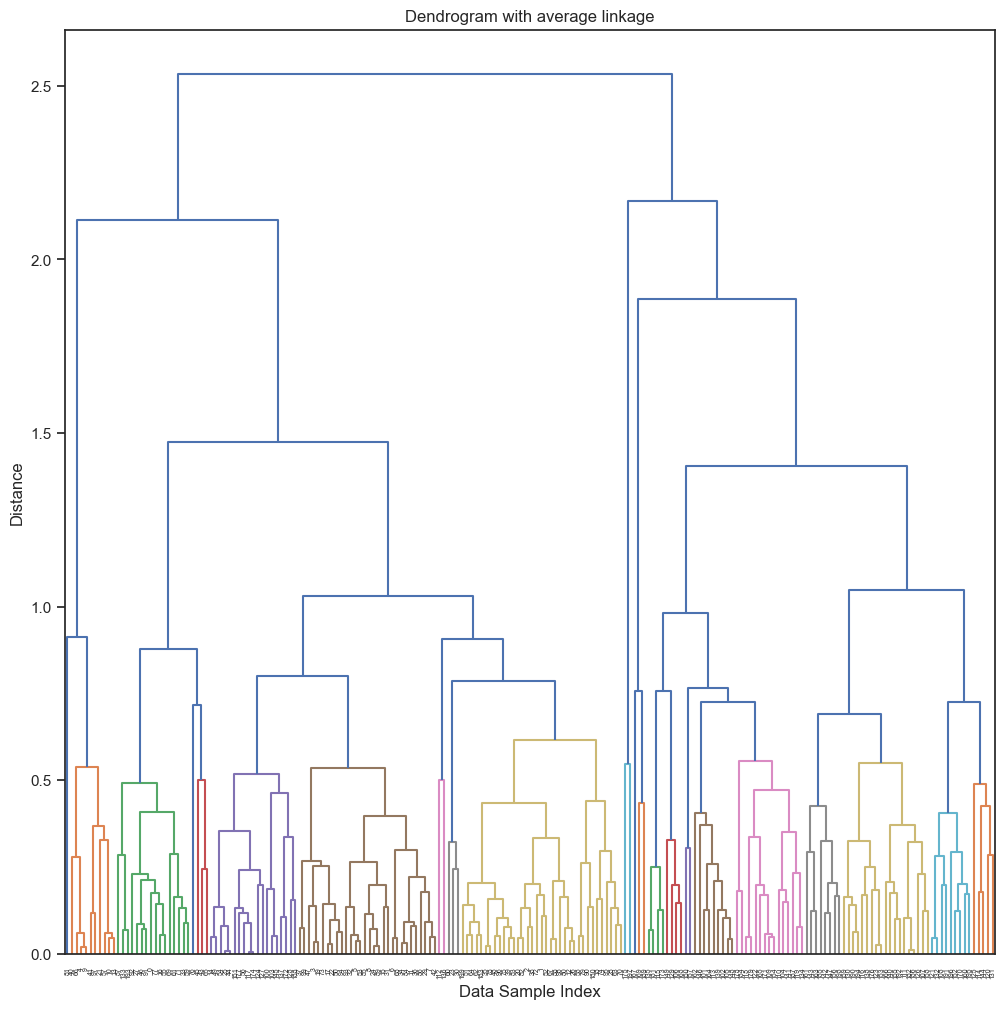
Now that we have explored the structure of the data and built some intuition on how many clusters and the distribution of the data samples in the cluster.
Next, we choose a distance threshold and assign each data point to a cluster ID.
In Sci-kit learn, the entire algorithm is incorporated in the function AgglomerativeClustering sklearn doc here. The function still needs either a threshold distance or a number of cluster to perform the clustering and assign a cluster ID to each data sample.
#
from sklearn.cluster import AgglomerativeClustering
# Let's first find a reasonable distance threshod by precalculating the linkage matrix
Z = hierarchy.linkage(X, "average")
thresh = 0.85*np.max(Z[:,2])    # choose a threshold distance
print(thresh)
# design model
model = AgglomerativeClustering(distance_threshold=thresh,linkage="average", n_clusters=None)
# fit model and predict clusters on the data samples
clusterID=model.fit_predict(X)
2.1553671407878263
X
array([[ 1.43350268e+00, -1.66284056e+00],
       [ 2.59380863e+00, -5.63943160e-01],
       [ 2.42359606e+00, -5.65095025e-01],
       [ 2.32138028e+00, -8.89751882e-01],
       [ 3.08113310e+00,  5.31875618e-01],
       [ 1.67295307e+00, -1.06168176e+00],
       [ 1.76546160e+00, -1.46554711e+00],
       [ 1.87876889e+00, -1.16816806e+00],
       [ 1.72637647e+00, -9.02902726e-01],
       [ 3.09689906e+00,  5.40367004e-01],
       [ 3.64575262e+00,  8.45857469e-01],
       [ 1.76975214e+00, -1.21307490e+00],
       [ 2.76846118e+00, -2.54990193e-01],
       [ 3.68808391e+00,  8.59655748e-01],
       [ 1.87810165e+00, -6.73339668e-01],
       [ 1.87812831e+00, -9.38358033e-01],
       [ 1.41679880e+00, -1.46310032e+00],
       [ 2.18452379e+00, -7.81692591e-01],
       [ 2.33553382e+00, -1.47805102e-01],
       [ 2.29233218e+00, -8.73416701e-01],
       [ 2.39393795e+00, -4.28975461e-01],
       [ 3.66982019e+00,  5.41413700e-01],
       [ 2.18493938e+00, -7.55188227e-01],
       [ 3.27894486e+00, -2.31675465e-01],
       [ 1.68104510e+00, -8.63028776e-01],
       [ 1.84020133e+00, -5.30472588e-01],
       [ 2.73669760e+00, -2.70985658e-01],
       [ 1.26564294e+00, -1.46166602e+00],
       [ 2.65140128e+00,  5.80467402e-02],
       [ 1.95214107e+00, -1.16500907e+00],
       [ 3.05707018e+00, -1.34573837e-01],
       [ 1.85955127e+00, -8.04350267e-01],
       [ 1.63007403e+00, -1.09610147e+00],
       [ 1.06848084e+00, -1.46725669e+00],
       [ 1.70181608e+00, -1.28679745e+00],
       [ 2.21153578e+00, -4.68576456e-01],
       [ 1.80184096e+00, -1.28410467e+00],
       [ 2.10227580e+00, -1.05836797e+00],
       [ 2.49539290e+00, -5.42819812e-01],
       [ 2.24931771e+00, -3.64705215e-01],
       [ 3.33087274e+00,  3.64033033e-01],
       [ 3.30468018e+00,  8.53659577e-01],
       [ 1.84805874e+00, -1.13147540e+00],
       [ 6.60365269e-01, -1.80414214e+00],
       [ 1.84388478e+00, -5.38063281e-01],
       [ 1.17049426e+00, -2.15910416e+00],
       [ 1.28546337e+00, -1.38837774e+00],
       [ 2.32622034e+00, -1.01790279e+00],
       [ 2.30845379e+00, -3.10000543e-01],
       [ 1.83286861e+00, -6.60519969e-01],
       [ 2.08764086e+00, -8.31707406e-01],
       [ 2.05876537e+00, -3.07107204e-01],
       [ 2.56801387e+00, -4.57569875e-01],
       [ 1.64054926e+00, -1.04690610e+00],
       [ 1.91910361e+00, -5.53637802e-01],
       [ 1.42788150e+00, -1.51463199e+00],
       [ 1.72189621e+00, -3.66200710e-01],
       [ 3.63469071e+00,  8.98945863e-01],
       [ 2.90781154e+00,  2.14169642e-01],
       [ 1.00105924e+00, -1.52197574e+00],
       [ 3.16121009e+00,  1.19479893e-01],
       [ 9.53254559e-01, -1.39001736e+00],
       [ 2.15975960e+00, -3.82639626e-01],
       [ 2.56653506e+00,  8.89181306e-02],
       [ 2.08072608e+00, -3.55846061e-01],
       [ 8.70684726e-01, -1.92810648e+00],
       [ 3.11794405e+00,  4.84028749e-01],
       [ 2.55538743e+00, -3.01150443e-01],
       [ 1.73013118e+00, -1.49084638e+00],
       [ 1.20082908e+00, -1.68189771e+00],
       [ 2.48879817e+00,  1.15525786e-01],
       [ 9.58804467e-01, -1.59939861e+00],
       [ 2.61267658e+00, -6.75354527e-01],
       [ 2.09816631e+00, -6.59364427e-01],
       [ 2.49249982e+00, -1.60928335e-01],
       [ 2.24279855e+00, -3.07493105e-01],
       [ 5.40331959e-01, -2.52807567e+00],
       [ 1.55222759e+00, -1.54062965e+00],
       [ 2.23299271e+00, -4.72716534e-01],
       [ 2.85836044e+00,  2.06380531e-01],
       [ 2.79615554e+00, -2.03566152e-01],
       [ 4.21210983e+00,  1.03815835e+00],
       [ 2.38469443e+00, -4.74095585e-01],
       [ 2.27882059e+00, -3.98780850e-01],
       [ 1.71775288e+00, -1.26189863e+00],
       [ 1.69664895e+00, -7.59120796e-01],
       [ 2.06419769e+00, -1.20086303e+00],
       [ 1.05152703e+00, -1.18314361e+00],
       [ 2.57593123e+00, -3.36967973e-01],
       [ 1.66848983e+00, -8.44882771e-01],
       [ 2.75732367e+00,  4.07107968e-01],
       [ 1.34929719e+00, -1.41774748e+00],
       [ 1.54158392e+00, -1.36127618e+00],
       [ 1.52575621e+00, -1.01484245e+00],
       [ 2.11022491e+00, -7.73334082e-01],
       [ 2.67081402e+00, -8.59995190e-02],
       [ 2.33814553e+00, -2.70801967e-01],
       [ 3.34277804e+00,  7.41781333e-01],
       [ 2.73096308e+00, -3.99908489e-01],
       [ 2.07230686e+00, -9.89595643e-01],
       [ 1.77200563e+00,  2.99958587e-02],
       [-1.13559614e+00,  1.55258449e-01],
       [-1.11535082e+00,  3.08998769e-01],
       [ 1.59103728e+00, -4.29352404e-02],
       [-5.17002010e-01, -1.76323776e-01],
       [-1.18181892e+00,  3.90535107e-01],
       [-6.52976973e-01,  7.52854687e-01],
       [ 7.21362874e-01, -2.99549186e-01],
       [ 1.79905757e-01, -3.16827078e-01],
       [-7.15547294e-01,  8.33613971e-02],
       [-3.28597742e-01, -1.42373896e-01],
       [ 4.53120750e-01,  3.15607835e-02],
       [ 2.22140377e+00,  3.01317991e-01],
       [-9.68179228e-01,  3.74368878e-01],
       [ 6.55799770e-01, -7.20555138e-01],
       [ 4.91468729e-02,  7.54375250e-01],
       [ 1.03494963e-01,  2.59265875e-01],
       [ 1.64575823e+00, -4.05394413e-01],
       [-9.50274156e-01, -7.57472288e-02],
       [-3.92742328e-01,  1.28344035e-01],
       [ 3.24402698e-01, -1.18035155e+00],
       [-1.22872158e-01, -3.69104212e-01],
       [-8.58464736e-01,  1.29739056e-01],
       [ 2.60605548e-01,  1.27723895e-01],
       [ 1.50654833e+00, -5.47691796e-01],
       [ 3.56598296e-01, -5.04798007e-01],
       [ 5.28566571e-01, -3.48948642e-01],
       [ 1.42892166e+00, -3.65958117e-01],
       [ 1.27481244e+00, -4.35171223e-01],
       [-6.51344574e-01,  9.60009622e-01],
       [ 3.89813112e-01,  1.93205588e-01],
       [ 3.65301846e-01, -8.99702835e-01],
       [-1.45044537e-01, -4.07132985e-01],
       [ 1.24893725e+00, -1.02294638e+00],
       [-3.28855255e-01,  1.71049697e-01],
       [-2.80752904e-02,  5.10116954e-01],
       [ 1.75642317e+00,  4.88678261e-01],
       [ 1.29385795e+00, -1.03337844e-01],
       [ 2.37029163e-02,  1.09091501e-01],
       [-1.17675743e+00,  4.72706875e-01],
       [ 1.00157524e+00, -1.10487413e-02],
       [-4.70089548e-01, -3.53575704e-02],
       [ 7.34510049e-01,  3.55729680e-01],
       [ 1.13571728e+00,  3.17468526e-01],
       [ 6.90950553e-01, -8.94288096e-01],
       [ 1.62941687e+00, -7.67580740e-02],
       [-1.45789629e+00,  2.48032570e-01],
       [ 7.05010276e-01,  4.69039912e-01],
       [-1.20158980e+00,  3.53412077e-01],
       [-7.35469237e-01,  1.16392710e+00],
       [-1.12263265e+00, -4.10420561e-01],
       [ 1.69033981e+00, -2.66887625e-01],
       [-2.69490068e-01, -7.40928480e-01],
       [ 2.35235665e-01,  1.26122375e-01],
       [-6.83847536e-01,  4.72048413e-02],
       [ 8.68738041e-01, -1.08537423e-01],
       [ 9.01008876e-01,  4.70308463e-01],
       [-1.40079389e+00, -2.84583932e-01],
       [ 7.20269556e-01, -1.77578831e-01],
       [ 5.19274190e-01,  3.33992835e-01],
       [-1.13058067e-01, -5.65073966e-01],
       [ 1.20159493e+00,  5.69565340e-01],
       [-1.15089793e+00,  6.88499613e-01],
       [ 1.23605235e+00,  2.47963855e-01],
       [-1.00917668e+00,  1.46473182e-01],
       [-6.39975399e-01,  2.35710083e-01],
       [ 7.70832949e-01,  1.00380339e-01],
       [-1.77784322e+00, -9.93289237e-01],
       [-7.80046686e-01,  8.21236235e-01],
       [-1.14262720e+00, -1.03501758e+00],
       [-1.47855870e-01, -7.44265462e-01],
       [-6.59461729e-01,  9.65681801e-02],
       [ 1.31478216e+00,  1.31240204e-03],
       [-7.34913307e-02,  7.24248697e-01],
       [ 1.64228344e+00, -4.10013437e-01],
       [-2.23062432e+00,  1.04984011e+00],
       [ 2.78193582e-01, -5.18092002e-02],
       [ 1.58428941e+00, -3.24568202e-01],
       [-6.91949590e-01, -4.70130848e-01],
       [-9.97071249e-01, -8.43585916e-02],
       [ 2.63412378e+00,  3.55567437e-01],
       [-9.61819897e-02,  4.99918722e-01],
       [ 5.04767375e-01, -6.00113409e-02],
       [ 2.14118360e+00, -3.32081209e-01],
       [-5.19876832e-01, -4.18712198e-01],
       [ 8.61971214e-01,  7.04966072e-01],
       [ 5.09478493e-01, -5.14403563e-02],
       [-1.46903645e-01,  2.37813526e-01],
       [ 1.18381967e+00, -3.11049848e-01],
       [-1.03058095e+00, -1.45270114e+00],
       [ 3.57949544e-01,  3.03760092e-01],
       [ 1.82903172e-02, -2.02642287e-01],
       [ 8.20002856e-01, -2.08593236e-02],
       [ 1.31551975e+00, -1.00896047e+00],
       [ 3.89098648e-01,  3.59051900e-01],
       [-2.85451879e-01, -5.73109557e-01],
       [ 6.98750850e-02, -7.10184613e-01],
       [-1.81970102e+00,  6.89038735e-01],
       [ 8.95239386e-01,  3.06025041e-01],
       [ 1.98100851e+00, -2.93914670e-01]])
plt.scatter(X[:,0],X[:,1],c=clusterID)
<matplotlib.collections.PathCollection at 0x2bc2b4eb0>
Geosciences Applications
In the following exercise, we will try to find clusters from features of a set of seismic waveforms. THe waveforms come from Mt Hood, an ice-capped volcano in the Cascades that experience seismic events from the volcanic acticities (magmatic and hydrothermal), tectonic context, and glacier/snow related seismic events.
PCA before clustering#
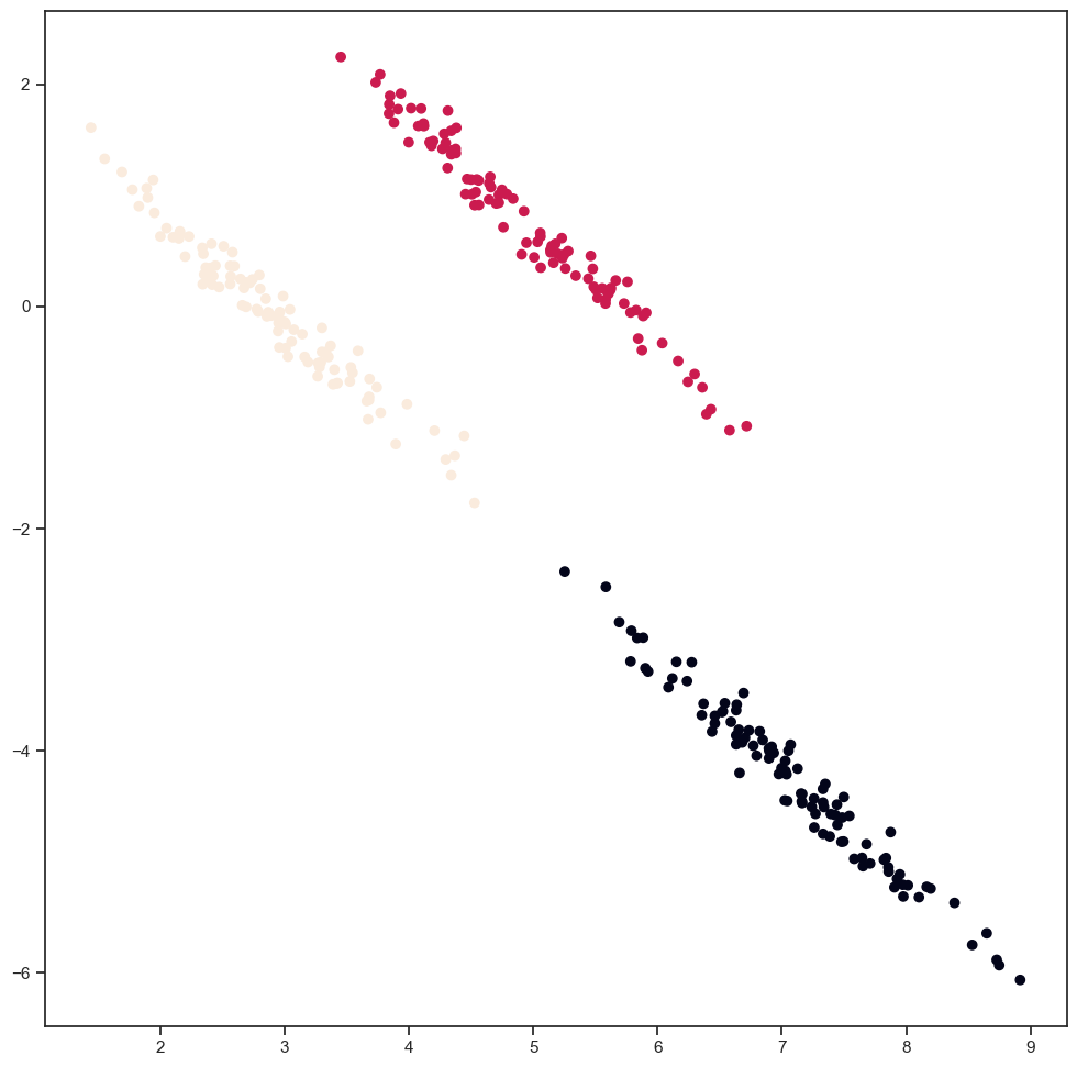
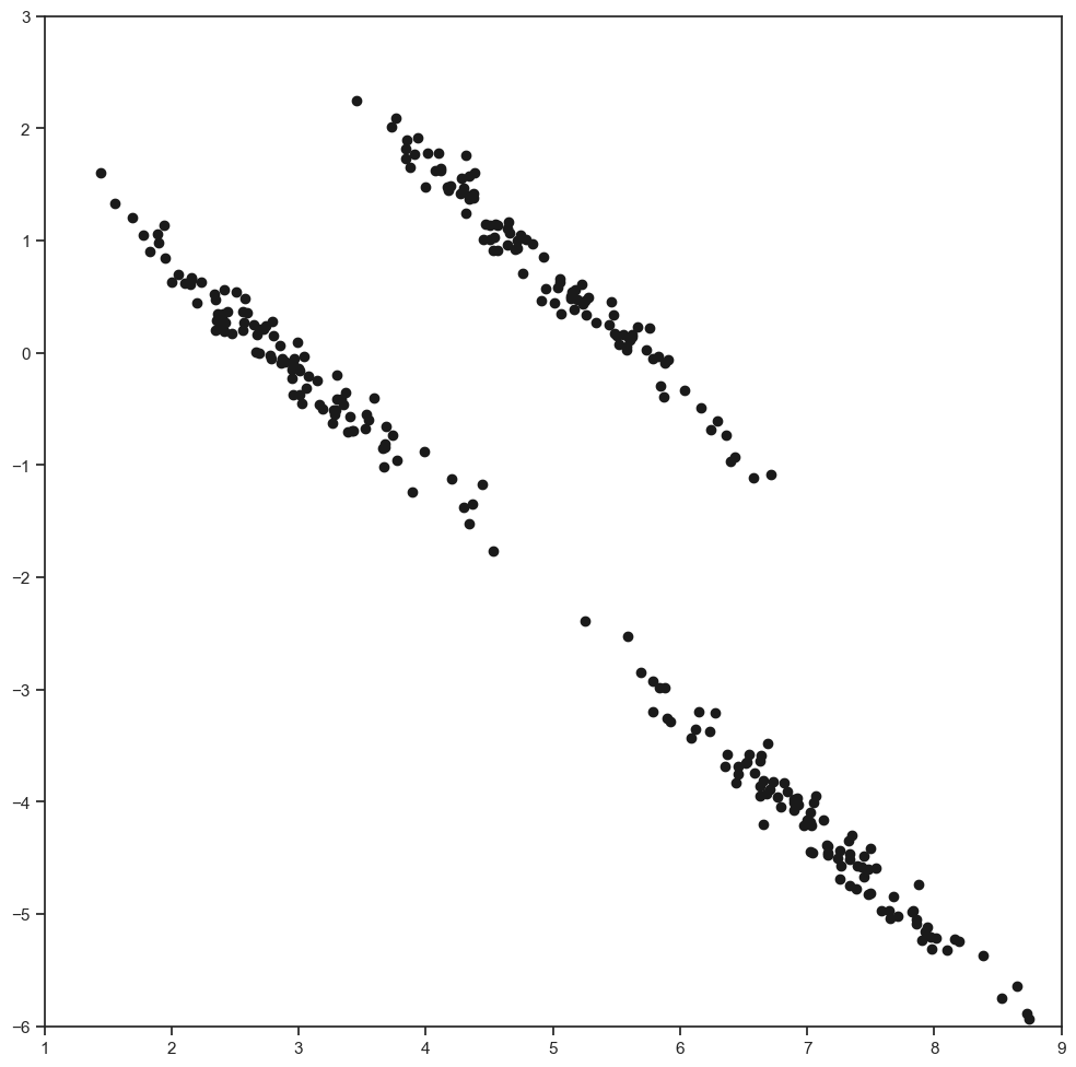
Let us generate synthetics data.
centers = np.array([[2, 2], [2, 8], [4, 3]])
radius = [0.1, 1]
synthetics = np.empty([0, 2])
for i in range(0, 3):
    X = centers[i, 0] + radius[0] * np.random.randn(100)
    Y = centers[i, 1] + radius[1] * np.random.randn(100)
    U = (X + Y) * sqrt(2) / 2
    V = (X - Y) * sqrt(2) / 2
    synthetics = np.concatenate([synthetics, np.vstack((U, V)).T])
plt.plot(synthetics[:,0], synthetics[:,1], 'ko')
plt.xlim(1, 9)
plt.ylim(-6, 3)
(-6.0, 3.0)
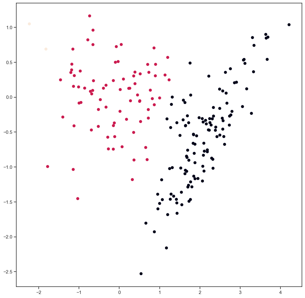
Let us now do k-means clustering with 3 clusters.
random.seed(0)
(clusters, objective, centers) = my_kmeans(synthetics, 3)
plt.scatter(synthetics[:,0], synthetics[:,1], c=clusters)
<matplotlib.collections.PathCollection at 0x2bdd92640>
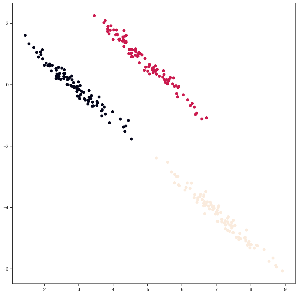
What happens if we apply PCA + normalization before the clustering?
pca = PCA(n_components=2)
synthetics_pca = pca.fit_transform(synthetics)
scaler = preprocessing.StandardScaler().fit(synthetics_pca)
synthetics_scaled = scaler.transform(synthetics_pca)
(clusters, objective, centers) = my_kmeans(synthetics_scaled, 3)
plt.scatter(synthetics[:,0], synthetics[:,1], c=clusters)
<matplotlib.collections.PathCollection at 0x2bde1d5e0>