4.5 The Three Pillars of Model Development

A working deep learning model rests on three pillars:

1. Training data: its quality, diversity, balance among classes, and noise level.
2. Architecture: the family of functions the network can represent, and how many parameters it spends doing so.
3. Training strategy: the loss function, the optimizer, the learning rate, the batch size, the stopping rule.

Most model failures trace back to exactly one of these pillars, and each pillar fails with a recognizable signature. This notebook is a hands-on lab: we hold one classification task fixed and break each pillar on purpose, so you learn to read the signatures before you meet them in your project data.

The lab uses small multi-layer perceptrons on a synthetic lithology table. Every experiment runs in seconds on a laptop CPU. You can raise sample counts and epochs on your own machine; the lessons do not change.

🖥️ Lecture slides — Session 24 — lab I (Wed Nov 25)

🖥️ Lecture slides — Session 25 — lab II (Mon Nov 30)

1. One task, one small model¶

The task for the whole lab: classify rock samples into three lithology classes (granite, basalt, andesite) from 9 geochemical and physical features (major-element oxides in wt%, density in g/cm³, magnetic susceptibility in SI units). The data comes from mlgeo_synth.geochem_table, a generator that plants realistic correlations between oxides through a latent differentiation index. Because the generator is ours, we control the exact amount of label noise, class imbalance, and sensor noise — the knobs real data never gives us.

One adjustment makes the lab realistic: the generator’s raw tables are almost perfectly separable, which no field instrument delivers. Every dataset in this lab therefore carries a fixed measurement-noise floor of one standard deviation per feature, applied to training, validation, and test alike. The corruption experiments in Section 3 add specific defects on top of that floor.

1.1 Train, validation, and test sets¶

Before any experiment, the data is split three ways:

• Training set: used to fit the model. It should be the largest portion, typically 60-80% of the data, and as diverse and balanced as the problem allows.
• Validation set: used during training to tune hyperparameters and detect overfitting. It gives an estimate of performance on unseen data while decisions are still being made. Typically 10-20%.
• Test set: used once, at the end, to report generalization. It must stay completely separate from every decision made during model development. If information from the test set influences training or model selection, the reported performance is inflated. This failure is called data leakage, and it appears again in Section 5.

One detail matters for this lab: our test set is always clean (no label noise, no defects beyond the shared measurement-noise floor), even when we corrupt the training data on purpose. That is how we measure what corruption costs.

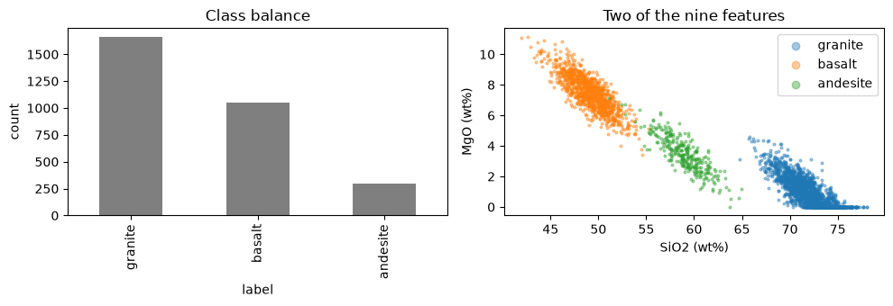
The classes are imbalanced by construction (andesite is rare) and they overlap in feature space. Both properties are typical of geochemical classification problems.

1.2 Lab helpers¶

Three pieces of code carry the whole lab: a data function with corruption knobs, a configurable MLP, and a training loop that records learning curves. Read them once, carefully; every experiment below is a few lines that call them.

A note on the training loop: it samples a fresh random minibatch each step (minibatch stochastic gradient descent, Section 2.4) and records train and validation loss once per epoch, evaluated in eval() mode on the full splits. Those two curves per run are the diagnostic instrument for the entire lab.

2. What training minimizes¶

Before the experiments, the vocabulary. A loss function measures how far the model’s predictions are from the labels. It provides the single number that gradient descent pushes downhill, so its choice shapes everything the network learns. Loss functions $\mathcal{L}(\mathbf{y}, \mathbf{\hat{y}}, \mathbf{w})$ quantify the residuals between ground-truth labels $\mathbf{y}$ and predictions $\mathbf{\hat{y}}$, and they must be differentiable with respect to the model parameters $\mathbf{w}$.

2.1 Losses for regression¶

• Mean squared error penalizes large errors quadratically. It is the natural choice when errors are close to Gaussian:

  $\mathrm{MSE} = \frac{1}{m} \sum_{i=1}^m \left( \hat{y}_i - y_i \right)^2$

• Mean absolute error penalizes large errors less, which suits heavy-tailed error distributions. Its gradient has constant magnitude, which can slow convergence near the minimum; adaptive optimizers such as Adam mitigate this:

  $\mathrm{MAE} = \frac{1}{m} \sum_{i=1}^m |\hat{y}_i - y_i|$

• Huber loss switches between the two: quadratic for errors smaller than a threshold δ (smooth gradients near the minimum), linear beyond it (outliers do not dominate).

2.2 Losses for classification¶

Binary classifiers output a probability through the logistic sigmoid $\sigma(x) = 1/(1 + e^{-x})$ and train with the binary cross-entropy:

$\mathcal{L}(\mathbf{w}) = - \frac{1}{m} \sum_{i=1}^m \left[ y_i \log \hat{p}_i + (1 - y_i) \log(1 - \hat{p}_i) \right]$

For $K$ classes, the network outputs one score $s_k$ per class and the softmax converts scores to probabilities:

$\hat{p}_k = \frac{\exp(s_k)}{\sum_{j=1}^K \exp(s_j)}$

with the multi-class cross-entropy as the loss. PyTorch’s nn.CrossEntropyLoss applies the softmax internally, which is why our MLP outputs raw logits.

2.3 Geoscience-aware losses¶

Standard losses miss objectives that matter in our field. Because any differentiable function of predictions can be a loss term, we can encode those objectives directly:

• Class weighting for rare events. Earthquakes, landslides, and rock-fall signals are rare classes; weighting their errors more (nn.CrossEntropyLoss(weight=...)) keeps the optimizer from ignoring them. Section 3.2 shows why this matters.

• Waveform similarity. A network that reconstructs seismograms should match wiggle for wiggle. Adding a correlation-coefficient term rewards phase alignment that MSE barely sees:

  $\mathcal{L}(\mathbf{\hat{u}}, \mathbf{u}) = \mathrm{MSE}(\mathbf{\hat{u}}, \mathbf{u}) + \lambda \left(1 - \mathrm{CC}(\mathbf{\hat{u}}, \mathbf{u})\right)$

• Physics constraints. When the output is a physical field, a loss term can penalize violations of a governing equation (conservation of mass, a heat equation residual). This is the basis of physics-informed neural networks, notebook 4.7.

• Uncertainty-aware losses. Probabilistic forecasts train with negative log-likelihood, which penalizes both over- and under-confidence.

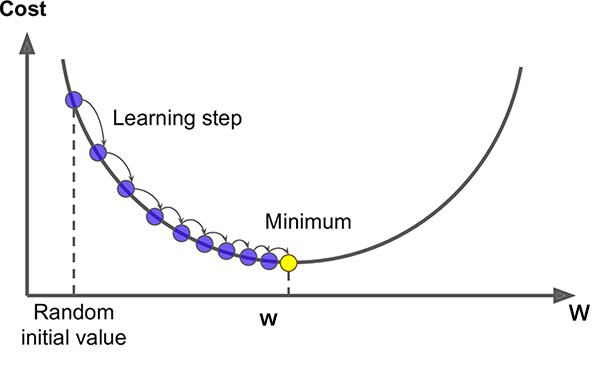
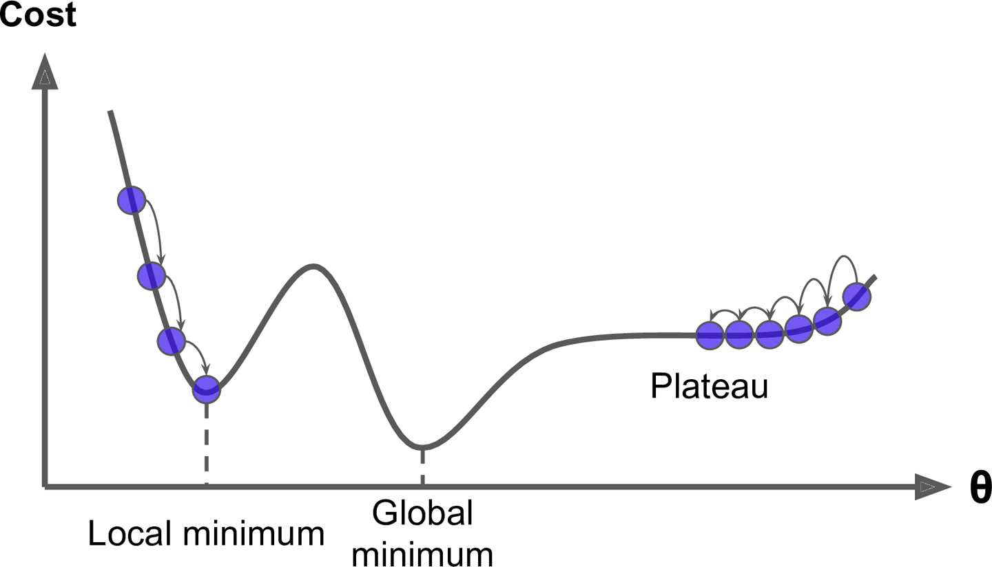
2.4 Gradient descent and the learning rate¶

Training updates the parameters in the direction that reduces the loss:

$w_j^{(k+1)} = w_j^{(k)} - \alpha \frac{\partial \mathcal{L}}{\partial w_j}$

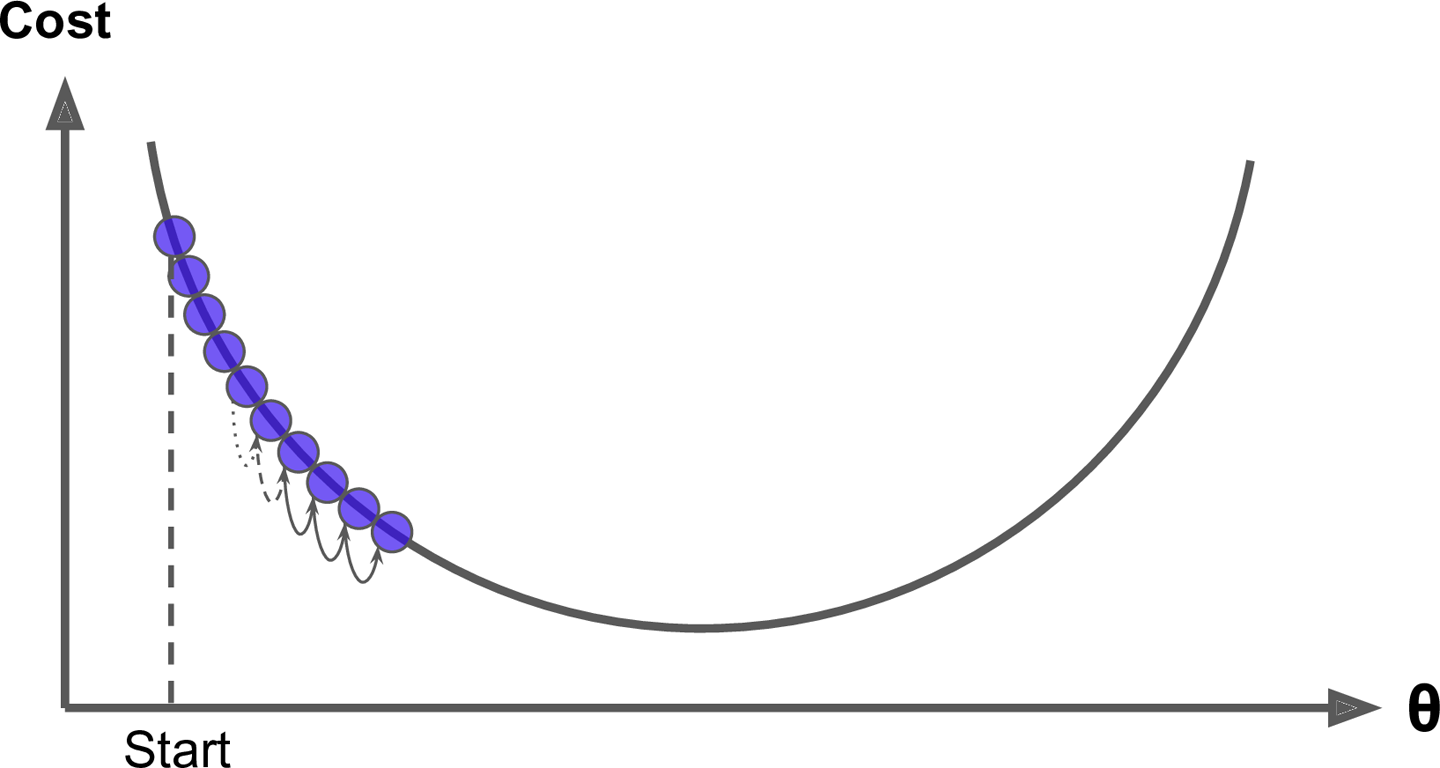
where α is the learning rate, the single most consequential hyperparameter in this notebook.

Gradient descent on a convex, well-behaved loss.	A poorly behaved loss with local minima.

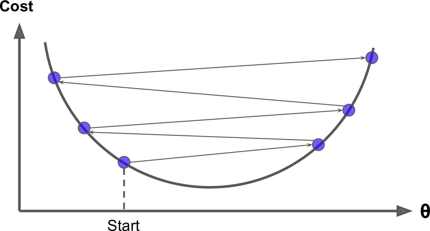α too small: convergence crawls.	α too large: steps overshoot the minimum.

Three variants differ in how much data each update sees:

• Batch gradient descent uses the full training set per step: exact gradients, expensive steps.
• Stochastic gradient descent (SGD) uses one sample per step: cheap, noisy updates, sensitive to feature scaling.
• Minibatch gradient descent uses a small random subset per step. This is the standard in deep learning, and what our train_model does. The batch size trades gradient noise against step cost; Section 5.2 measures the effect.

Adaptive optimizers (Adam, RMSProp) rescale each parameter’s step using running gradient statistics. Adam is the default in this course.

2.5 Bias, variance, underfitting, overfitting¶

Generalization error decomposes into three parts:

• Bias: error from wrong model assumptions (fitting a line to a curve). High bias shows up as high loss on the training data itself.
• Variance: error from excessive sensitivity to the particular training samples. High variance shows up as a gap between training and validation loss.
• Irreducible error: noise in the data. No model removes it; only better data does (fix sensors, remove outliers — Pillar 1).

Underfitting = high bias: both training and validation losses plateau at a high value. Remedies: bigger model, better features, less regularization.

Overfitting = high variance: training loss keeps falling while validation loss stalls and then climbs. The model has started to memorize noise. Remedies: more data, a smaller model, regularization, early stopping.

A rule worth memorizing: you do not know whether you can overfit until you do. Grow the model until it overfits, then back off or regularize. Both signatures appear in real curves in Section 5.

2.6 Regularization¶

Regularization constrains a flexible model to behave more simply:

• L2 penalty (ridge): add $\lambda \frac{1}{2} \lVert \mathbf{w} \rVert_2^2$ to the loss, shrinking all weights. In PyTorch optimizers this is the weight_decay argument.
• L1 penalty (lasso): add $\lambda \lVert \mathbf{w} \rVert_1$, which drives unimportant weights to exactly zero — a form of feature selection.
• Elastic net: a weighted combination of both.
• Dropout: randomly zero a fraction of activations during training, so no unit can rely on specific partners. Used in notebook 4.2 and available as a knob in our MLP.
• Early stopping: stop training when validation loss stops improving (Section 5.3).
• Data augmentation: enlarge and diversify the training set with transformed copies (shifts, added noise). It regularizes through the data pillar rather than the model.

3. Pillar 1 — Training-data curation¶

Model quality starts in the data, and no architecture or optimizer rescues a corrupted training set. Because our generator controls the corruption exactly, we can measure what each defect costs. In every experiment the test set stays clean, so the curves isolate the effect of training-data quality.

3.1 Label noise¶

Real labels are wrong more often than we like to admit: analyst picks disagree, catalogs inherit historical errors, field classifications get revised. We flip a fraction of training labels at random and retrain — in two data regimes, because the answer depends on how much data you have. Each point averages three seeds.

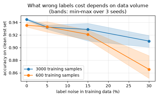
Two regimes, two stories. With 3000 training samples, even 30% of randomly flipped labels costs little: cross-entropy averages over many samples, the flips are symmetric, and the correct majority still pins down the class boundaries. With 600 samples the same model has enough capacity to memorize the flipped labels instead of averaging them away, and accuracy falls several points. Label noise is most dangerous exactly where geoscience usually lives: small labeled datasets and models large enough to memorize them. The shaded bands are the min-max spread over the three seeds — the run-to-run variability that a single-seed experiment hides. Read the bands before trusting any difference between two points: where the bands overlap, the difference may be initialization luck, not the knob you turned. Here the spread is not decoration: at 3000 samples the three seeds span up to 0.028 (at 15% noise) — most of the 0.035 that separates the clean and 30%-noise means — so a single-seed version of this figure could have told nearly any story. Every summary number in this lab that comes from repeated runs is now reported with its seed span..

What to look for in real data. Validation accuracy that plateaus below what the class overlap suggests is a label-quality symptom, not an architecture problem. To detect it: inspect the samples the model gets most confidently “wrong” (they are often mislabeled, not misclassified), have a second analyst relabel a random subset and measure agreement, and cross-check labels against independent catalogs. And remember the noise that does the damage in practice is rarely symmetric: an analyst who systematically confuses two signal types biases the boundary itself, which is far worse than random flips — the next experiment measures exactly that. Fixing a thousand labels usually beats adding a million parameters.

3.2 Class imbalance¶

Andesite is already the rare class. We now shrink it further and watch per-class recall, not overall accuracy.

Structured disagreement: when the errors have a pattern¶

Uniform random flips are the kindest possible label error, and the experiment above shows why: with enough data they average away. Real label errors come from people, and people disagree in patterns. We simulate a field campaign mapped by two geologists who split the area between them. Each mislabels 30% of their samples — the same total error rate as the harshest uniform experiment above — but their confusions are never random: granite slides to andesite, basalt slides to andesite, andesite to either neighbor. Nobody ever calls a basalt a granite. The confusion concentrates between adjacent lithologies on the differentiation axis, which is exactly how real mapping disagreement behaves.

Same 3000-sample regime, same model, same training budget; only the error pattern changes.

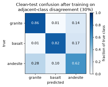
Same error rate, three times the damage: 30% uniform flips cost 3.5 accuracy points (0.945 to 0.910), 30% adjacent-class disagreement costs 12.5 (0.945 to 0.820), and no seed comes close to closing the gap (best seed 0.850). The confusion matrix shows where the points went. Both mappers dump their errors into “andesite”, so the model has learned an andesite class that annexes the boundary zones of its neighbors: 14% of true granites and 16% of true basalts now come back “andesite”, while true andesite recall falls to 0.61. And this is the 3000-sample regime — the one where uniform flips were nearly free.

This result matters far beyond this notebook, so here it is without the code. Every label in a geoscience dataset is an interpretation, not a measurement. A geologic map records what one mapper concluded from outcrops, float, and judgment calls at contacts; a seismic phase pick records where one analyst decided the wave arrived; a landslide inventory records which slope features one interpreter accepted as failures. Send two qualified experts over the same ground, the same waveforms, or the same imagery independently and they will disagree — most often between adjacent categories: granodiorite versus granite, Pn versus P, old landslide versus hummocky moraine. That disagreement is measurable (double-map a subset, double-pick a day of records) and is routinely a two-digit percentage at the category boundaries.

Structured disagreement hurts more than random error because it votes coherently. A thousand random flips scatter in all directions and cancel; a thousand adjacent-class confusions all push the same class boundary the same way, so more data makes the model more confident in the mappers’ shared mistake, not less. The practical consequence: inter-rater agreement is a ceiling on the accuracy any model can demonstrate, because the model is graded against labels that carry the disagreement. Before spending a month on architectures, spend a day measuring how often two experts agree on your labels — that number tells you when to stop tuning and start relabeling.

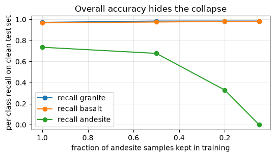
Read the two columns against each other. Overall accuracy drifts down a few points — nothing alarming on a dashboard. Andesite recall collapses to zero: the model has stopped predicting the class entirely. Notice also that even at full data the rare class starts disadvantaged (recall 0.74 against 0.97 for the majority classes). This is the most common silent failure in geoscience classification, where the rare class (the eruption, the induced event, the landslide) is the one you care about.

What to look for in real data. Always report the full confusion matrix and per-class recall; never accuracy alone. If the minority class matters, use class weights in the loss, oversample it, or generate augmented minority examples — and check that the fix shows up in recall, not just in the loss.

3.3 Sensor noise on the features¶

Now the labels are right but the instrument degrades: we add extra Gaussian noise to the training and validation features, on top of the shared 1.0σ measurement floor, in units of one feature standard deviation. The test set keeps the normal floor — this simulates training on data from a worse sensor than the one you deploy.

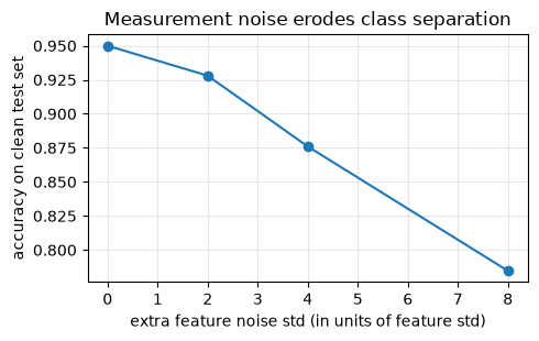
Once the added noise reaches a few times the natural spread of each feature, the class clusters smear into each other and accuracy slides toward chance. No model recovers separation that the measurements no longer contain — this is the irreducible-error term of Section 2.5 made visible.

What to look for in real data. Estimate measurement uncertainty per feature (repeat measurements, instrument specifications, calibration records) and compare it against the between-class separation of that feature. Features whose noise exceeds their class separation add no signal; cleaning or dropping them is data curation, not defeat.

3.4 How much data is enough?¶

The classic learning-curve diagnostic plots performance against training-set size. This is the function to reuse whenever someone asks “would more data help?” — a question better measured than debated.

Heteroscedastic quality: when you know how noisy each sample is¶

The sweep above degraded every sample equally. Real tables mix provenances: half your geochemistry from a laboratory XRF with tight analytical error, half from a portable field unit several times worse — and the metadata usually says which is which, because analytical uncertainty is reported per sample. (Sensor streams do the same thing in time: mlgeo_synth.degrade_series returns a per-sample sigma_mm column for exactly this reason.) Noise whose variance changes from sample to sample is called heteroscedastic, and it is the aleatoric half of the uncertainty vocabulary from lesson 3.9: randomness in the measurement itself, which no amount of training data removes — but which you can refuse to treat as truth.

The standard cross-entropy treats every sample as equally trustworthy. If the variance is known, the fix is to weight each sample’s loss by the inverse of its variance ($w_i \propto 1/\sigma_i^2$), the classification analogue of weighted least squares. We measure what ignoring the metadata costs and what the weights recover: each training sample draws its noise floor from {0.5, 4.0} standard deviations with equal probability (lab-grade or field-grade), and the same model trains once without the weights and once with them.

The mixed-quality table costs 1.7 points against the all-lab-grade reference (0.933 vs 0.950). Handing the model the variance it already had in the metadata recovers 1.3 of them (0.946) — no new data, one line of loss code — and the seed bands of the two schemes do not overlap (0.932-0.935 vs 0.939-0.951), so the gain is not initialization luck.

What to look for in real data. Any column named uncertainty, std_err, quality, or pick_weight is an invitation to weight the loss — seismic catalogs, geochemical databases, and GNSS solutions all ship one, and most pipelines drop it at ingest. Down-weighting is also the honest alternative to the tempting shortcut of deleting the noisy half: the field-grade samples still carry signal, just less of it per sample, and the weights price that in.

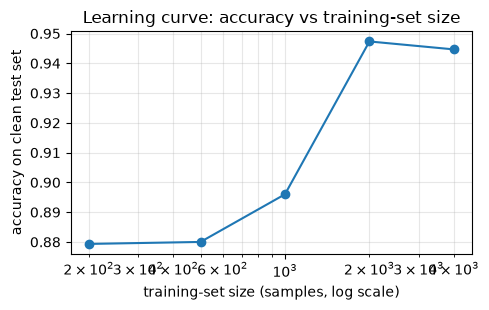
The curve rises steeply, then flattens: past a few thousand samples, more identical data buys little. If the curve is still rising at your current data size, collect more data before tuning anything else. If it has flattened, more of the same data will not help; better labels, better features, or harder examples might.

4. Pillar 2 — Architecture¶

With the data held clean and fixed, we now vary the model. The questions are always the same: how wide, how deep, and compared to what baseline?

4.1 Width¶

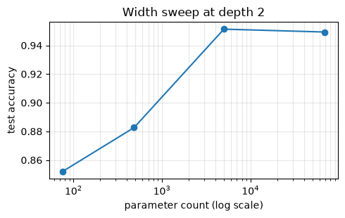
Accuracy saturates within a factor of a few of the smallest adequate width. Past that point, parameters are free in accuracy but not in training time, memory, or overfitting risk on smaller datasets.

4.2 Depth at a fixed parameter budget¶

Is it better to spend a fixed parameter budget on depth or width? We solve for the width that gives each depth roughly the same parameter count, then compare.

On a 9-feature tabular problem, depth buys little: the correlations the generator planted are low-order, and a shallow-but-wide network represents them as well as a deep one. Depth pays when the data has hierarchical structure — edges to textures to objects in images (notebook 4.3), samples to motifs to phrases in sequences (notebook 4.4). Match the architecture to the structure of the data, not to fashion.

4.3 The baseline you must always run¶

Every deep model needs a cheap reference point. For classification, that is multinomial logistic regression — equivalently, our MLP with depth 0 (a single linear layer plus softmax).

The gap is real but modest — typical for well-behaved tabular data. If your deep model cannot beat the linear baseline, the problem is the data or the features, not a missing layer. Report the baseline in every project; it is the honest denominator for every claim about deep learning.

4.4 Deep ensembles: uncertainty from disagreement¶

Train the same architecture from several random seeds and the runs converge to different functions that agree on easy samples and disagree near class boundaries. That disagreement is a practical uncertainty signal (Lakshminarayanan et al., 2017, NeurIPS), and it costs nothing but repeated training. Whether the signal is any good is not something to assert; it splits into two measurable claims. Discrimination: does disagreement rank samples by their risk of error? Calibration: when the ensemble says 80%, is it right about 80% of the time? The two are independent — a model can rank its errors perfectly while every stated probability is 20 points too confident — and we measure both.

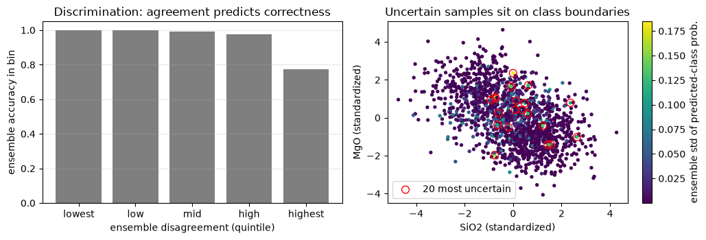
Two payoffs. First, the ensemble mean is usually at least as accurate as the best single member. Second — and more useful in practice — samples where the members disagree are exactly the samples the ensemble gets wrong most often, and they cluster along class boundaries in feature space. In a real workflow you would route the flagged samples to a human analyst. This is discrimination — the same skill the vote-spread of lesson 3.9 had, measured the same way: bin by the uncertainty score, check that accuracy falls across the bins. Nothing in this figure says whether the ensemble’s probabilities mean what they claim. The final-project milestone offers this analysis as one of the two required uncertainty experiments.

5. Pillar 3 — Training strategies¶

Same data, same architecture: everything below changes only how we train.

5.1 The learning rate, three ways¶

That second property is calibration, and it needs the tools from lesson 3.6: a reliability diagram on the ensemble-mean probabilities, summarized by the expected calibration error (ECE) — the average gap between stated confidence and observed accuracy, weighted by how many samples land in each confidence bin. For a 3-class problem the predicted-class confidence lives between 1/3 and 1, so the bins do too. We compare the ensemble mean against a single member to see what averaging buys.

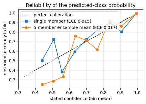
The measurement corrects the claim an earlier draft of this section made. Lakshminarayanan et al. (2017) found that deep ensembles improve calibration, and on deep networks — especially under distribution shift — they generally do. Here the single member is already nearly calibrated (ECE 0.015) and the ensemble mean gains nothing measurable (ECE 0.017; both curves hug the diagonal). A two-layer MLP on nine features with a 1σ noise floor is not miscalibrated enough to fix. “Well calibrated” is a measurement you attach to a model after running this cell, not an adjective that comes bundled with a method.

Keep the two diagnostics distinct in your write-ups. The quintile plot answers “can I trust the ranking?” — useful for routing samples to an analyst, where only the order matters. The reliability diagram answers “can I trust the number?” — required whenever the probability itself feeds a decision threshold someone else owns, the situation lesson 3.6 warned about. Reporting one as evidence for the other is the exact error this section originally contained, and it survives peer review depressingly often.

4.5 MC dropout: a second uncertainty method from one model¶

Five training runs is a real cost when one run takes a week. Monte Carlo dropout buys an uncertainty estimate from a single trained model: train with dropout as usual (the knob our MLP has carried since Section 2.6), then at prediction time leave dropout on and run the same input through the network $T$ times. Each pass samples a different random subnetwork; the mean over passes is the prediction and the spread over passes is the uncertainty — an approximation to Bayesian inference over the weights (Gal & Ghahramani, 2016, ICML).

The honest comparison is head-to-head on the same data and the same test set: one dropout model with $T=50$ stochastic passes against the 5-member ensemble, scored on accuracy, calibration (ECE), and discrimination (spread-vs-error), with the cost stated next to the numbers.

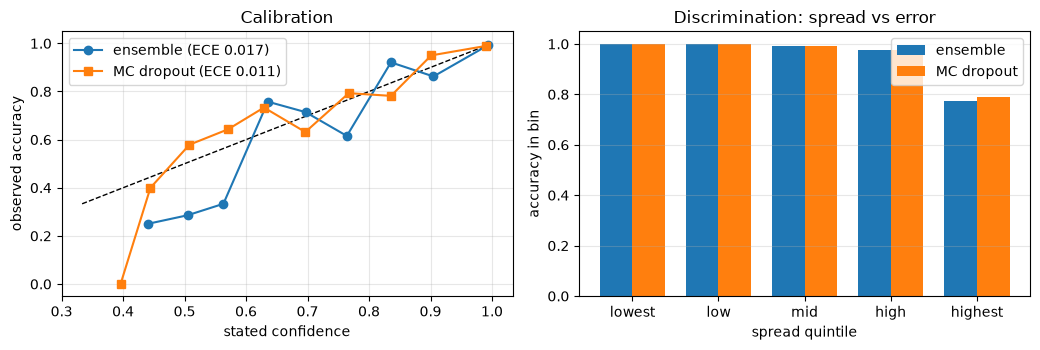
The numbers refuse to crown the expensive method. MC dropout matches the ensemble on accuracy (0.952 vs 0.949 — a difference inside the seed spread of a single run), edges it on calibration (ECE 0.011 vs 0.017), and draws the same discrimination curve (accuracy in the highest-spread quintile 0.79 vs 0.77; the other four quintiles agree to three decimals) — for one training run instead of five. The 50 prediction passes are the cheap side of the ledger; the training runs are the expensive one. On this task, one dropout model is the rational choice. The reasons the ensemble survives in practice sit outside this table: its documented calibration advantage appears on large networks under distribution shift, its members train in parallel while dropout passes at scale can bottleneck inference, and its disagreement comes from genuinely independent solutions — the property we now take out of range.

4.6 Out of range: interpolation, extrapolation, and what disagreement can flag¶

Every score in this notebook so far shares a hidden assumption: the test set was drawn from the same generator, over the same parameter ranges, as the training set. The model interpolates — it predicts inside the region of feature space its training data covered. Deployment breaks the assumption routinely: the mapped area ends, the next pluton is more evolved than anything in the survey, the new station sits on softer ground. Predicting there is extrapolation, and lesson 3.8 showed with its ladder of splits that interpolation and extrapolation are different claims — the split you choose decides which claim your score supports. Here we watch one model cross the line, and ask the operational question: does ensemble disagreement warn us when it happens?

The setup uses the generator’s own hidden knob. Each sample’s oxides are driven by a latent differentiation index (Section 1); its observable proxy is the per-class standardized SiO₂. We train an ensemble only on samples within one standard deviation of each unit’s typical composition — the field campaign mapped only typical granites, typical basalts, typical andesites — then evaluate on a fresh draw spanning the full range, including the evolved and primitive extremes the model has never seen.

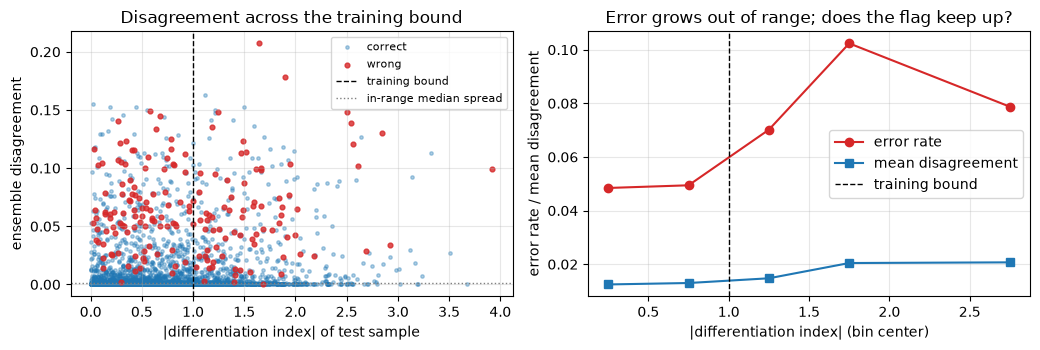
Read the table first. The error rate nearly doubles across the training bound — 4.9% in range, 8.0% just past it, 8.5% beyond two units — a gradual failure, because an unusually evolved granite is still mostly granite-like. Mean disagreement rises with it, 0.013 to 0.021: the ensemble notices. And of the 77 out-of-range errors, exactly one is a silent failure — wrong, with disagreement at or below the in-range median. That single sample is the mechanism to memorize: an extreme composition that landed inside a neighboring class’s familiar territory, so all five members confidently agreed on the same wrong label. Disagreement flags unfamiliar regions of feature space; it cannot flag a sample whose label changed while its features came to look familiar. Under a larger shift, that one sample becomes a population.

The scatter adds the second caution: the in-range and out-of-range disagreement distributions overlap heavily. The mean rises 60%, but no threshold on the spread reconstructs the training bound — the bound is metadata that only you have, which is why it must be stated, not inferred from the model’s behavior.

Your training distribution is a contract. Every number this lab produced — accuracy, ECE, the quintile plots — is a term of that contract, valid for samples drawn from the ranges the training data covered. Outside those ranges the model is extrapolating, and no diagnostic computed inside the range certifies what it does out there. State the range alongside the model whenever you release one, and treat predictions beyond it as unwarranted until out-of-range labels say otherwise.

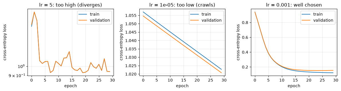
Three signatures to memorize:

• Too high: the loss oscillates or explodes; each step overshoots the valley. (With unstable runs the loss can reach inf or NaN; the log axis makes the explosion readable.)
• Too low: both curves creep down a nearly straight line and training “works” but would need hundreds of epochs.
• Well chosen: fast early drop, then a smooth flattening.

When in doubt, sweep the learning rate in powers of 10 first. Nothing else in this section matters until this is roughly right.

5.2 Batch size¶

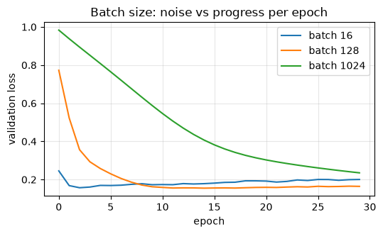
Small batches take many noisy steps per epoch: fast initial progress and a mild regularizing effect, at the price of jitter. Large batches take few smooth steps: each epoch does less, so at a fixed epoch budget the curve lags, and very large batches often generalize slightly worse. Batch size also sets memory use, which is what usually decides it on real hardware. The common practice: the largest batch that fits comfortably in memory, with the learning rate re-tuned when the batch changes.

5.3 Overfitting live, and early stopping¶

To force overfitting we give a large model a small, noisy training set and let it run long.

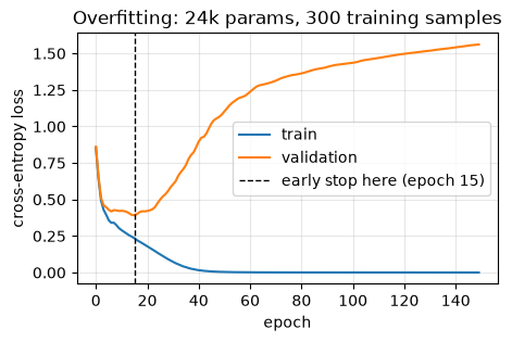
The textbook signature: training loss falls toward zero while validation loss bottoms out and climbs. Early stopping regularizes by simply keeping the model from the epoch where validation loss was lowest. The standard implementation keeps a patience counter:

best_val, patience, wait = float("inf"), 20, 0
for epoch in range(max_epochs):
    train_one_epoch(...)
    val = validation_loss(...)
    if val < best_val:
        best_val, wait = val, 0
        torch.save(model.state_dict(), "best.pt")   # checkpoint the best model
    else:
        wait += 1
        if wait > patience:
            break                                    # stop; reload best.pt

Notebook 4.2 covers the checkpointing half of this pattern.

5.4 Learning-rate schedulers¶

A schedule starts with a large learning rate for fast progress and shrinks it for a precise finish — a compromise between the “too high” and “too low” panels of Section 5.1.

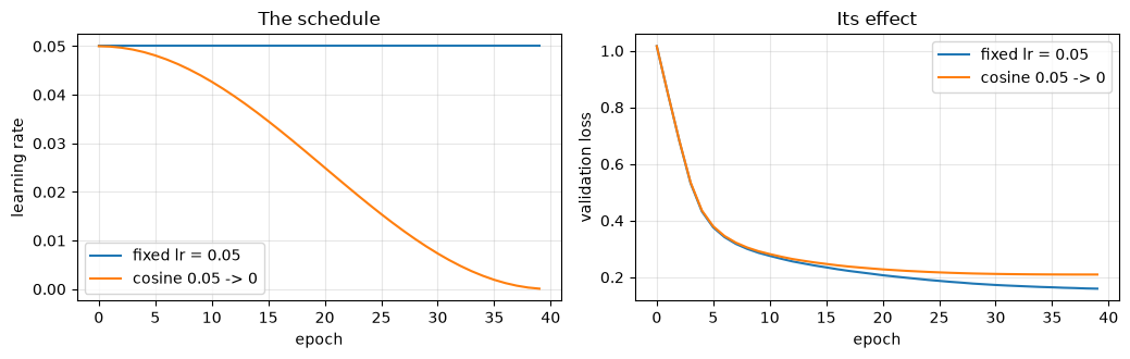
StepLR (drop the rate by a factor every $k$ epochs) and cosine annealing are the two schedules you will meet most often. On a problem this small the gain is modest; on large models, schedules are standard practice.

5.5 Exercise: diagnose six broken training runs¶

Below are learning curves from six training runs, each broken in a different way (or suspicious in a different way). The pathologies, in shuffled order: learning rate too high, learning rate too low, overfitting, underfitting (not enough capacity), heavy label noise, and data leakage into the validation set.

Diagnose each run from its curves before reading the generation code above the figure or opening the solution.

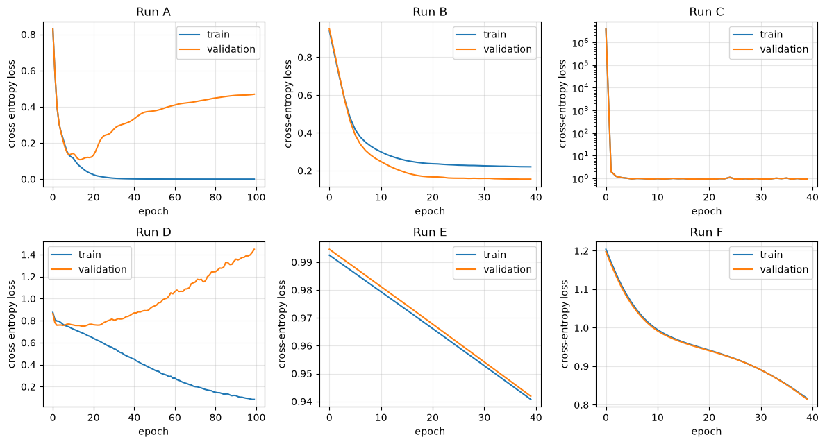
For each run, write down: the pathology, the evidence in the curves, and the fix you would try first.

5.6 Hyperparameter search with Optuna¶

After the manual sweeps, the systematic version. Optuna samples hyperparameter combinations, observes the validation score of each trial, and focuses the search where scores are good. Twenty trials on our small task take under a minute.

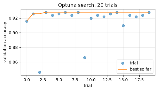
Search the hyperparameters that Section 5 showed matter — learning rate first, then regularization and width — over ranges your manual sweeps found sensible. Always keep the final test set out of the search: Optuna optimizes the validation score, and the test set is spent only once at the end.

5.7 Why architecture search stopped mattering¶

Ten years ago, neural architecture search — algorithms that design network wiring automatically — was an active research front. It has largely faded, for a simple reason: a handful of canonical architectures (the MLP, the convolutional network, the transformer) plus scale won. In domain after domain, taking a standard architecture and spending the compute on more data, more parameters, and better training beat bespoke wiring discovered by search. What remains of the search problem moved to where you just practiced it: hyperparameters (Optuna and its relatives) and, above all, the data pillar. This is also the practical advice for your projects: pick the canonical architecture that matches your data’s structure, then spend your effort on data curation and training diagnostics.

6. Checklist for training a deep learning model¶

1. Characterize the data (Chapter 2): dimensionality, units, correlations, class balance.
2. Set aside the test data first. Consider causality and independence between test and training samples: random splits leak when samples are correlated in time or space.
3. Curate the training data (Pillar 1): audit labels, quantify measurement noise, check per-class counts, and diversify with augmentation where physical transformations make sense.
4. Design the network (Pillar 2): match the architecture family to the structure of the data, start small, and always include the linear or classical-ML baseline.
5. Define the loss appropriate to the task and the domain objectives (Section 2), consulting the PyTorch loss-function documentation and scikit-learn metrics.
6. Choose the optimizer and training strategy (Pillar 3): Adam as a default, learning rate swept in powers of ten, the largest comfortable batch, a scheduler for longer runs.
7. Train with diagnostics on: record training and validation curves every run, checkpoint the best validation model, early-stop when validation stalls.
8. Evaluate honestly: per-class metrics, the untouched test set once, an uncertainty estimate (a deep ensemble if you can afford five runs, MC dropout if you cannot), a calibration check on any probability you report (Section 4.4), and a statement of the training ranges outside which none of the numbers apply (Section 4.6).

7. Summary¶

You now have a diagnostic vocabulary attached to curves you have generated yourself: what label noise — random and structured — class imbalance, and sensor noise — uniform and heteroscedastic — cost (Pillar 1); how width, depth, baselines, ensembles, and MC dropout behave, how calibration differs from discrimination, and what happens out of range (Pillar 2); and what learning rate, batch size, overfitting, early stopping, and schedulers look like in learning curves (Pillar 3). The six broken runs of Section 5.5 are the exam that real projects will keep administering.

Apply this lab to your own project: for the final-project milestone you will reuse the sweep patterns on your architectures, keep a diagnostics appendix with at least one failed run, and run either the deep-ensemble analysis from Section 4.4 or the fine-tuning experiment from notebook 4.6.