Forecasting means predicting future values of a time series from its past. Geoscience runs on forecasts: atmospheric CO2, river discharge, glacier flow, groundwater levels, space weather. This notebook is a forecasting shootout. We take the canonical model families you have met in this book, point them all at the same two real data sets, evaluate them with the same metrics on the same temporal split, and let a comparison table decide.
The contestants, in order of increasing complexity:
- Baselines: naive persistence and seasonal naive. Always first.
- SARIMA: a classical statistical model (
statsmodels). - Gradient boosting on lag features (
lightgbm): classic ML from Chapter 3, adapted to time. - A small LSTM (
torch): the recurrent architecture from notebook 4.4. - A small transformer encoder (
torch): the attention pattern from notebook 4.4.
The data:
- Mauna Loa monthly CO2 (NOAA Global Monitoring Laboratory): long, regular, strongly seasonal, with a smooth trend. The friendly case, and the primary benchmark.
- Jakobshavn Isbrae surface speed (Greenland): short, irregularly sampled, noisy. The hard case.
Learning goals
- Split time series data temporally and explain why random splits leak future information.
- Build lag features that use only the past.
- Evaluate forecasts with MSE, RMSE, MAE, MAPE, and MASE, computed in code.
- Turn a point forecaster into a probabilistic one with the pinball loss, then verify it: empirical coverage of the 90% interval, and CRPS.
- Measure how forecast error grows with lead time and locate the skill horizon.
- Quantify how much a model ranking moves across random seeds, and score rare events separately from the bulk.
- Judge when model complexity pays off and when a baseline wins.
The notebook ends with a class leaderboard in two tracks: a public CO2 forecast that is a diagnostic only (Section 7 explains why it is trivially gameable, and why we say so in print), and a hidden synthetic series that carries the grading weight.
import os
import warnings
from pathlib import Path

import numpy as np
import pandas as pd
import matplotlib.pyplot as plt
import pooch
import torch
import torch.nn as nn

import mlgeo_synth

np.random.seed(0)
torch.manual_seed(0)

device = torch.device("cuda" if torch.cuda.is_available()
                      else "mps" if torch.backends.mps.is_available()
                      else "cpu")
print("device:", device)

# One fixed color per model, reused in every figure (Okabe-Ito palette, colorblind-safe).
COLORS = {
    "observations":   "#000000",
    "naive":          "#999999",
    "seasonal naive": "#E69F00",
    "SARIMA":         "#0072B2",
    "ARIMA":          "#0072B2",
    "LightGBM":       "#009E73",
    "LSTM":           "#D55E00",
    "Transformer":    "#CC79A7",
}
plt.rcParams.update({"figure.dpi": 100, "axes.grid": True, "grid.alpha": 0.3})
device: cpu
1. Data
1.1 Mauna Loa monthly CO2
The Mauna Loa record is the longest continuous direct measurement of atmospheric CO2, started by Charles Keeling in 1958. NOAA GML distributes monthly means in a text file: about 42 lines of # comments, one header line, then whitespace-delimited columns (year, month, decimal date, monthly average in ppm, deseasonalized value, number of days, standard deviation, uncertainty). We fetch it with pooch, which caches the file locally.
co2_url = "https://raw.githubusercontent.com/UW-MLGEO/MLGeo-dataset/main/data/data_co2.csv"
co2_file = pooch.retrieve(co2_url, known_hash=None, fname="data_co2.csv")

co2 = pd.read_csv(co2_file, comment="#", sep=r"\s+", header=0)
co2.columns = ["year", "month", "decimal_date", "average",
               "deseasonalized", "ndays", "stdev", "unc"]
co2.index = pd.to_datetime(co2["year"].astype(str) + "-"
                           + co2["month"].astype(str).str.zfill(2))
y_full = co2["average"].astype("float64")
print(y_full.shape, "monthly values,", y_full.index[0].date(), "to", y_full.index[-1].date())
Downloading data from 'https://raw.githubusercontent.com/UW-MLGEO/MLGeo-dataset/main/data/data_co2.csv' to file '/home/runner/.cache/pooch/data_co2.csv'.
SHA256 hash of downloaded file: 871222f3f96a85edcbeeca8a5cc5beb7f8df1f20c9fb9cdcf98a186ecc3c32d1
Use this value as the 'known_hash' argument of 'pooch.retrieve' to ensure that the file hasn't changed if it is downloaded again in the future.
(798,) monthly values, 1958-03-01 to 2024-08-01
1.2 The leaderboard holdout: hands off the last 12 months
Before any modeling, we remove the final 12 months of the record: 2023-09 through 2024-08. These months are the class leaderboard holdout (Section 7) — a test set we will score exactly once. Nothing in the modeling sections touches them: no plot, no fit, no metric. We keep only their dates.
holdout_months = y_full.index[-12:]
y = y_full.iloc[:-12].copy()
del y_full  # the holdout values are gone from this notebook

assert holdout_months[0] == pd.Timestamp("2023-09-01")
assert holdout_months[-1] == pd.Timestamp("2024-08-01")
print("holdout months:", holdout_months.strftime("%Y-%m").tolist())
print("working series:", y.index[0].date(), "to", y.index[-1].date(), f"({len(y)} months)")
holdout months: ['2023-09', '2023-10', '2023-11', '2023-12', '2024-01', '2024-02', '2024-03', '2024-04', '2024-05', '2024-06', '2024-07', '2024-08']
working series: 1958-03-01 to 2023-08-01 (786 months)
fig, axes = plt.subplots(1, 2, figsize=(10, 3.2))
axes[0].plot(y.index, y.values, color=COLORS["observations"], lw=1)
axes[0].set_title("Mauna Loa CO$_2$, full record")
axes[1].plot(y.loc["2013":].index, y.loc["2013":].values,
             color=COLORS["observations"], lw=1.2)
axes[1].set_title("Last decade")
for ax in axes:
    ax.set_xlabel("year")
    ax.set_ylabel("CO$_2$ (ppm)")
fig.tight_layout()
plt.show()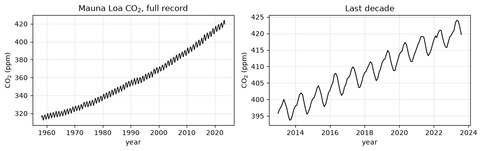
A smooth accelerating trend plus a sawtooth annual cycle (northern-hemisphere vegetation draws down CO2 each summer). Highly predictable structure. Any model that cannot beat “repeat last year’s shape” here should embarrass its author.
1.3 Jakobshavn Isbrae surface speed
Jakobshavn Isbrae in west Greenland is one of the fastest glaciers on Earth. The file holds satellite-derived surface speed (m/yr) for a 10 x 10 pixel patch near the terminus, sampled irregularly (every 6 to 12 days) since 2015. Missing values are coded as -1.0; we mask them to NaN and average the valid pixels at each date into one mean-speed series.
ice_url = "https://raw.githubusercontent.com/UW-MLGEO/MLGeo-dataset/main/data/data_ice_jakobshavn.csv"
ice_file = pooch.retrieve(ice_url, known_hash=None, fname="data_ice_jakobshavn.csv")

ice_raw = pd.read_csv(ice_file, parse_dates=["Date"]).set_index("Date")
ice_raw = ice_raw.where(ice_raw != -1.0)          # -1.0 means missing
ice = ice_raw.mean(axis=1).dropna()               # patch mean over valid pixels
print(ice.shape, "samples,", ice.index[0].date(), "to", ice.index[-1].date())
print("median sampling interval:", ice.index.to_series().diff().median())

fig, ax = plt.subplots(figsize=(9, 3))
ax.plot(ice.index, ice.values, color=COLORS["observations"], lw=1)
ax.set_xlabel("year")
ax.set_ylabel("surface speed (m/yr)")
ax.set_title("Jakobshavn Isbrae, patch-mean surface speed")
fig.tight_layout()
plt.show()
Downloading data from 'https://raw.githubusercontent.com/UW-MLGEO/MLGeo-dataset/main/data/data_ice_jakobshavn.csv' to file '/home/runner/.cache/pooch/data_ice_jakobshavn.csv'.
SHA256 hash of downloaded file: 22fe5834937c549b6e6ef4eee74a157239c0601952e456d1fc8b7005a95e5e15
Use this value as the 'known_hash' argument of 'pooch.retrieve' to ensure that the file hasn't changed if it is downloaded again in the future.
(430,) samples, 2015-01-01 to 2024-04-13
median sampling interval: 6 days 00:00:00
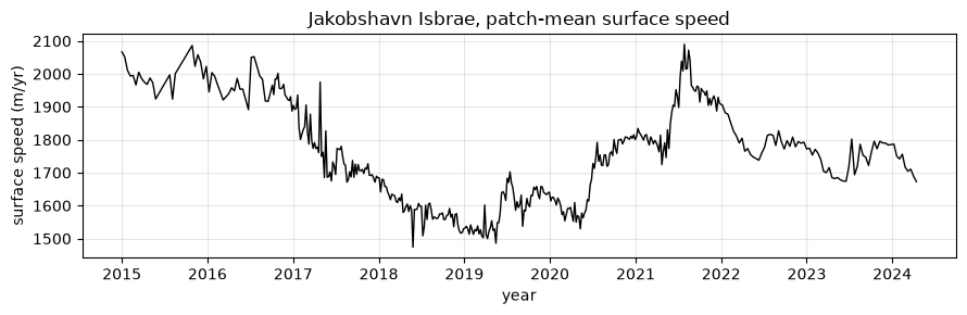
Summer speed-ups ride on top of multi-year swings tied to terminus position and ocean forcing. Compared with CO2 this series is short (about 430 samples over nine years), irregularly sampled, and its variability is not dominated by a clean repeating cycle.
2. Evaluation protocol
2.1 Temporal splits, identical for every model
A forecast model is only tested fairly on data from after everything it was trained on. A random train/test split of time series rows lets the model interpolate between neighbors of the test points, which inflates scores and predicts nothing. Every model below uses exactly these splits:
- CO2: TEST = the final 48 months of the working series, 2019-09 through 2023-08. TRAIN = everything before, 1958-03 through 2019-08.
- Ice: TEST = the final 20% of dates. TRAIN = the first 80%.
All models forecast the full test window in one go (a 48-month horizon for CO2), with no peeking at test values along the way.
H_CO2 = 48
train_co2, test_co2 = y.iloc[:-H_CO2], y.iloc[-H_CO2:]
assert test_co2.index[0] == pd.Timestamp("2019-09-01")
assert test_co2.index[-1] == pd.Timestamp("2023-08-01")

n_test_ice = int(0.2 * len(ice))
train_ice, test_ice = ice.iloc[:-n_test_ice], ice.iloc[-n_test_ice:]

print(f"CO2 : train {train_co2.index[0].date()} .. {train_co2.index[-1].date()} "
      f"({len(train_co2)}), test {test_co2.index[0].date()} .. {test_co2.index[-1].date()} ({len(test_co2)})")
print(f"ice : train {train_ice.index[0].date()} .. {train_ice.index[-1].date()} "
      f"({len(train_ice)}), test {test_ice.index[0].date()} .. {test_ice.index[-1].date()} ({len(test_ice)})")
CO2 : train 1958-03-01 .. 2019-08-01 (738), test 2019-09-01 .. 2023-08-01 (48)
ice : train 2015-01-01 .. 2021-09-20 (344), test 2021-09-26 .. 2024-04-13 (86)
2.2 Metrics
With forecast errors over the test points:
- MSE . Penalizes large errors quadratically; units are squared, so it is awkward to read.
- RMSE . Back in data units; still dominated by the largest errors.
- MAE . Data units, treats all errors linearly. Easiest to interpret.
- MAPE . Unit-free percent, but it blows up near zero values and is asymmetric (over-forecasts and under-forecasts are penalized differently). Fine for CO2 (~420 ppm) and ice speed, useless for series that cross zero.
- MASE (mean absolute scaled error): MAE divided by the MAE of the naive one-step forecast () on the training data. MASE means the model beats naive persistence at its own one-step game; MASE means a “repeat the last value” rule was better. It is unit-free, defined at zero, and comparable across series, which is why the class leaderboard uses it.
One helper computes all five. Every number in the comparison tables comes out of this function. Never type metric values into a table by hand; the 2024 edition of this notebook did, and the table was wrong.
def forecast_metrics(y_true, y_pred, y_train):
    """All metrics for one forecast. MASE is scaled by the training
    MAE of the naive one-step forecast (y_hat_t = y_{t-1})."""
    y_true = np.asarray(y_true, dtype=float)
    y_pred = np.asarray(y_pred, dtype=float)
    e = y_true - y_pred
    mse = np.mean(e**2)
    mae = np.mean(np.abs(e))
    naive_train_mae = np.mean(np.abs(np.diff(np.asarray(y_train, dtype=float))))
    return {"MSE": mse,
            "RMSE": np.sqrt(mse),
            "MAE": mae,
            "MAPE (%)": 100 * np.mean(np.abs(e / y_true)),
            "MASE": mae / naive_train_mae}

results_co2, preds_co2 = {}, {}   # metrics and predictions, filled model by model
results_ice, preds_ice = {}, {}

def register(results, preds, name, y_pred, test, train):
    preds[name] = np.asarray(y_pred, dtype=float)
    results[name] = forecast_metrics(test.values, y_pred, train.values)
    print(name, "->", {k: round(v, 3) for k, v in results[name].items()})
3. The shootout on CO2
3.1 Baselines first, always
- Naive persistence: repeat the last training value across the whole 48-month horizon.
- Seasonal naive: repeat the last 12 training months, tiled four times. This copies last year’s seasonal shape but freezes the trend.
If a model cannot beat these, its complexity bought nothing.
naive = np.full(H_CO2, train_co2.iloc[-1])
seasonal = np.tile(train_co2.values[-12:], H_CO2 // 12)

register(results_co2, preds_co2, "naive", naive, test_co2, train_co2)
register(results_co2, preds_co2, "seasonal naive", seasonal, test_co2, train_co2)
naive -> {'MSE': np.float64(56.38), 'RMSE': np.float64(7.509), 'MAE': np.float64(6.679), 'MAPE (%)': np.float64(1.596), 'MASE': np.float64(6.09)}
seasonal naive -> {'MSE': np.float64(41.971), 'RMSE': np.float64(6.478), 'MAE': np.float64(5.961), 'MAPE (%)': np.float64(1.427), 'MASE': np.float64(5.436)}
3.2 SARIMA
SARIMA (seasonal ARIMA) models the differenced series with autoregressive and moving-average terms, plus seasonal counterparts at lag 12. We use the standard textbook order for Mauna Loa, : one regular difference for the trend, one seasonal difference for the annual cycle. We cap the optimizer iterations to keep the fit fast; this is a benchmark entry, not a tuning exercise.
from statsmodels.tsa.statespace.sarimax import SARIMAX

with warnings.catch_warnings():
    warnings.simplefilter("ignore")
    sarima = SARIMAX(train_co2, order=(1, 1, 1),
                     seasonal_order=(1, 1, 1, 12)).fit(disp=False, maxiter=50)
sarima_pred = sarima.forecast(H_CO2).values
register(results_co2, preds_co2, "SARIMA", sarima_pred, test_co2, train_co2)
SARIMA -> {'MSE': np.float64(0.129), 'RMSE': np.float64(0.359), 'MAE': np.float64(0.281), 'MAPE (%)': np.float64(0.067), 'MASE': np.float64(0.256)}
3.3 Gradient boosting on lag features
Tree ensembles know nothing about time. We hand them time explicitly, as a table where each row predicts one month from features built only from earlier months:
- lags 1, 2, 3, 6, 12, 24 (the value months before the target),
- the rolling mean of the 12 months before the target (i.e. shifted by one step so the target itself is excluded),
- the calendar month (known in advance, so it is fair game).
One subtlety: a regression tree predicts averages of training targets, so it can never output a value outside the range it saw in training. CO2 keeps rising past every training value, so a tree that predicts the level saturates near the training maximum and the forecast goes flat. The fix is to predict the one-month change and add it to the previous value; monthly changes are roughly stationary and sit well inside the training range. The features stay the same past-only lags.
The model predicts one step ahead. To cover the 48-month test window we forecast recursively: predict the next change, add it to the last value, append that prediction to the history, build features again, and so on. Errors compound, which is honest; the model gets no real observations from the test period.
from lightgbm import LGBMRegressor

def lag_feature_row(history, date, lags, roll):
    """Features for predicting the value at `date`, given all values before it."""
    row = {f"lag_{k}": history[-k] for k in lags}
    row[f"rollmean_{roll}"] = np.mean(history[-roll:])
    row["month"] = date.month
    return row

def build_training_table(series, lags, roll):
    """One row per predictable month; the target is the one-step change."""
    vals = series.to_numpy()
    start = max(max(lags), roll)          # first row with a full feature set
    rows = [lag_feature_row(vals[:i], series.index[i], lags, roll)
            for i in range(start, len(vals))]
    target = vals[start:] - vals[start - 1:-1]   # y_t - y_{t-1}
    return pd.DataFrame(rows), target

def lgbm_recursive_forecast(train_series, test_index, lags, roll, random_state=0):
    X_tr, y_tr = build_training_table(train_series, lags, roll)
    model = LGBMRegressor(n_estimators=300, learning_rate=0.05,
                          num_leaves=15, random_state=random_state, verbose=-1)
    model.fit(X_tr, y_tr)
    history = list(train_series.to_numpy())
    preds = []
    for date in test_index:               # recursive multi-step
        row = pd.DataFrame([lag_feature_row(np.asarray(history), date, lags, roll)])
        step = float(model.predict(row)[0])       # predicted change
        level = history[-1] + step
        preds.append(level)
        history.append(level)             # feed the prediction back in
    return np.array(preds), model
lgbm_pred_co2, _ = lgbm_recursive_forecast(train_co2, test_co2.index,
lags=[1, 2, 3, 6, 12, 24], roll=12)
register(results_co2, preds_co2, "LightGBM", lgbm_pred_co2, test_co2, train_co2)LightGBM -> {'MSE': np.float64(1.643), 'RMSE': np.float64(1.282), 'MAE': np.float64(1.03), 'MAPE (%)': np.float64(0.246), 'MASE': np.float64(0.939)}
3.4 A small LSTM
The deep models forecast directly: one forward pass maps a 36-month context window to all 48 horizon values at once (no recursion). Two practical points:
- Anchoring. CO2 trends upward forever, so test windows sit at levels the network never saw in training. We subtract the last context value (“anchor”) from each window, train on the anchored shapes, and add the anchor back to the prediction. The network learns change relative to now, which is stationary enough to generalize.
- Scaling. Anchored windows are divided by one global standard deviation from the training windows, keeping inputs O(1).
The model is small and trains for a few epochs; raise both on your own machine if you want.
def make_windows(values, context, horizon):
    """Anchored (context, horizon) windows: both parts minus the last context value."""
    X, Y = [], []
    for i in range(len(values) - context - horizon + 1):
        c = values[i:i + context]
        h = values[i + context:i + context + horizon]
        X.append(c - c[-1])
        Y.append(h - c[-1])
    return np.array(X, dtype=np.float32), np.array(Y, dtype=np.float32)

def train_forecaster(model, X, Y, epochs=40, lr=1e-3, batch_size=32):
    model.to(device)
    ds = torch.utils.data.TensorDataset(torch.from_numpy(X).unsqueeze(-1),
                                        torch.from_numpy(Y))
    dl = torch.utils.data.DataLoader(ds, batch_size=batch_size, shuffle=True)
    opt = torch.optim.Adam(model.parameters(), lr=lr)
    loss_fn = nn.MSELoss()
    losses = []
    for _ in range(epochs):
        model.train()
        total = 0.0
        for xb, yb in dl:
            xb, yb = xb.to(device), yb.to(device)
            opt.zero_grad()
            loss = loss_fn(model(xb), yb)
            loss.backward()
            opt.step()
            total += loss.item() * len(xb)
        losses.append(total / len(ds))
    return losses

def nn_forecast(model, context_values, scale):
    """Forecast one horizon from the last `context` observed values."""
    anchor = context_values[-1]
    x = torch.from_numpy(((context_values - anchor) / scale)
                         .astype(np.float32)).reshape(1, -1, 1).to(device)
    model.eval()
    with torch.no_grad():
        out = model(x).cpu().numpy().ravel()
    return out * scale + anchor
CONTEXT_CO2 = 36
Xc, Yc = make_windows(train_co2.to_numpy(), CONTEXT_CO2, H_CO2)
scale_co2 = float(Xc.std())
Xc, Yc = Xc / scale_co2, Yc / scale_co2
print(f"{len(Xc)} training windows, scale = {scale_co2:.2f} ppm")
class LSTMForecaster(nn.Module):
def __init__(self, horizon, hidden=32):
super().__init__()
self.lstm = nn.LSTM(input_size=1, hidden_size=hidden, batch_first=True)
self.head = nn.Linear(hidden, horizon)
def forward(self, x):
_, (h, _) = self.lstm(x)
return self.head(h[-1])
torch.manual_seed(0)
lstm_co2 = LSTMForecaster(horizon=H_CO2)
lstm_losses = train_forecaster(lstm_co2, Xc, Yc, epochs=40)
lstm_pred_co2 = nn_forecast(lstm_co2, train_co2.to_numpy()[-CONTEXT_CO2:], scale_co2)
register(results_co2, preds_co2, "LSTM", lstm_pred_co2, test_co2, train_co2)655 training windows, scale = 3.35 ppm
LSTM -> {'MSE': np.float64(1.085), 'RMSE': np.float64(1.042), 'MAE': np.float64(0.886), 'MAPE (%)': np.float64(0.212), 'MASE': np.float64(0.808)}
3.5 A small transformer encoder
Same windows, same anchoring, same direct multi-step head; only the sequence model changes. We reuse the pattern from notebook 4.4: project each scalar to a small embedding, add sinusoidal positional encoding (attention itself is order-blind), run two encoder layers, average over time, and map to the 48 horizon values.
class PositionalEncoding(nn.Module):
    def __init__(self, d_model, max_len=200):
        super().__init__()
        pos = torch.arange(max_len).unsqueeze(1).float()
        div = torch.exp(torch.arange(0, d_model, 2).float()
                        * (-np.log(10000.0) / d_model))
        pe = torch.zeros(max_len, d_model)
        pe[:, 0::2] = torch.sin(pos * div)
        pe[:, 1::2] = torch.cos(pos * div)
        self.register_buffer("pe", pe)
    def forward(self, x):                      # x: (batch, seq, d_model)
        return x + self.pe[: x.shape[1]]

class TransformerForecaster(nn.Module):
    def __init__(self, horizon, d_model=32, nhead=4, num_layers=2):
        super().__init__()
        self.embed = nn.Linear(1, d_model)
        self.pos = PositionalEncoding(d_model)
        layer = nn.TransformerEncoderLayer(d_model=d_model, nhead=nhead,
                                           dim_feedforward=64, dropout=0.1,
                                           batch_first=True)
        self.encoder = nn.TransformerEncoder(layer, num_layers=num_layers)
        self.head = nn.Linear(d_model, horizon)
    def forward(self, x):
        z = self.encoder(self.pos(self.embed(x)))
        return self.head(z.mean(dim=1))        # average over time steps

torch.manual_seed(0)
tfm_co2 = TransformerForecaster(horizon=H_CO2)
tfm_losses = train_forecaster(tfm_co2, Xc, Yc, epochs=40)
tfm_pred_co2 = nn_forecast(tfm_co2, train_co2.to_numpy()[-CONTEXT_CO2:], scale_co2)
register(results_co2, preds_co2, "Transformer", tfm_pred_co2, test_co2, train_co2)
Transformer -> {'MSE': np.float64(0.262), 'RMSE': np.float64(0.511), 'MAE': np.float64(0.401), 'MAPE (%)': np.float64(0.096), 'MASE': np.float64(0.366)}
fig, ax = plt.subplots(figsize=(6, 3))
ax.plot(lstm_losses, color=COLORS["LSTM"], lw=1.5, label="LSTM")
ax.plot(tfm_losses, color=COLORS["Transformer"], lw=1.5, label="Transformer")
ax.set_xlabel("epoch")
ax.set_ylabel("training MSE (scaled units)")
ax.set_yscale("log")
ax.set_title("Training loss, CO$_2$ deep models")
ax.legend()
fig.tight_layout()
plt.show()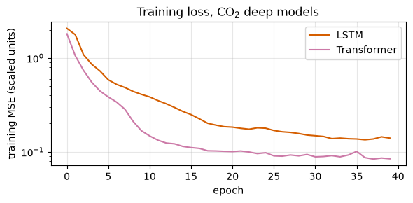
3.6 The comparison, computed honestly
The table below is built programmatically from results_co2, the dictionary that register() filled from the actual predictions. No number in it was typed by hand.
co2_table = pd.DataFrame(results_co2).T.sort_values("MASE").round(3)
co2_tablefig, ax = plt.subplots(figsize=(9, 4))
recent = y.loc["2017":]
ax.plot(recent.index, recent.values, color=COLORS["observations"],
lw=1.5, label="observations")
for name, pred in preds_co2.items():
ax.plot(test_co2.index, pred, color=COLORS[name], lw=1.2, ls="--", label=name)
ax.axvline(test_co2.index[0], color="0.6", lw=0.8)
ax.text(test_co2.index[0], ax.get_ylim()[1], " test window starts",
va="top", fontsize=8, color="0.4")
ax.set_xlabel("year")
ax.set_ylabel("CO$_2$ (ppm)")
ax.set_title("CO$_2$ test window: all forecasts vs observations")
ax.legend(fontsize=8, ncol=2)
fig.tight_layout()
plt.show()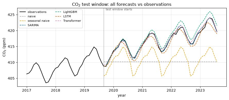
What to look for in your table and plot:
- Naive persistence ignores both trend and season; its flat line is the floor everyone should beat, and its MASE is large because a 48-month horizon is much harder than the one-step game MASE is scaled by.
- Seasonal naive copies the annual shape but freezes the trend, so it drifts below the observations by roughly the trend times the horizon. Still, it beats several trained models. That is the recurring lesson of forecasting benchmarks.
- SARIMA encodes exactly the two things this series is made of, a differenced trend and a 12-month cycle, in a handful of parameters. On this kind of series it is very hard to beat.
- LightGBM, LSTM, transformer must learn trend and season from examples. In a typical run all three reach MASE below 1 and land between the seasonal baseline and SARIMA; recursive feedback (LightGBM) and limited training data (the deep pair) both cost accuracy on a 4-year horizon. Model capacity is not the bottleneck; problem structure is.
3.7 From point forecasts to intervals: the pinball loss, coverage, and CRPS
Every model so far answers “what will CO2 be?” with one number per month. No serious user of a forecast settles for that: a reservoir operator, a carbon-budget analyst, and every operational weather center ask for the range of outcomes and how probable each is. The machinery is a small change to what we already have.
A model learns the quantile of the outcome when it is trained on the pinball loss (quantile loss)
which charges τ per unit of under-prediction and per unit of over-prediction; the minimizer of its expectation is exactly the τ-quantile. Predict and and you have a 90% prediction interval; is a median point forecast for free.
We give the LSTM from 3.4 a quantile head: instead of 48 numbers it emits — one per horizon step per quantile level — trained on the pinball loss averaged over levels. Same windows, same anchoring, same epochs. That buys us a verifiable claim, and verification is the point:
- Empirical coverage: over the 48 test months, how often does the observation actually fall inside the 90% interval? A calibrated forecast covers about 90%. Less means the model is overconfident; much more means the intervals are too wide to inform any decision. This is the same calibration discipline as the reliability curves of Chapters 3 and 4.5, applied to intervals.
- One wrinkle: quantile outputs trained independently can cross ( for some month). Sorting along the quantile axis at prediction time is the standard one-line repair, and we apply it below.
QUANTILES = np.round(np.arange(0.05, 0.951, 0.05), 2)   # 0.05, 0.10, ..., 0.95
N_Q = len(QUANTILES)
q_torch = torch.tensor(QUANTILES, dtype=torch.float32, device=device).view(1, 1, -1)

class QuantileLSTMForecaster(nn.Module):
    """The 3.4 LSTM with a (horizon x n_quantiles) head."""
    def __init__(self, horizon, n_q, hidden=32):
        super().__init__()
        self.horizon, self.n_q = horizon, n_q
        self.lstm = nn.LSTM(input_size=1, hidden_size=hidden, batch_first=True)
        self.head = nn.Linear(hidden, horizon * n_q)
    def forward(self, x):
        _, (h, _) = self.lstm(x)
        return self.head(h[-1]).view(-1, self.horizon, self.n_q)

def pinball_loss(pred, target):
    """Mean pinball loss over all quantile levels.
    pred: (batch, horizon, n_q); target: (batch, horizon)."""
    diff = target.unsqueeze(-1) - pred
    return torch.mean(torch.maximum(q_torch * diff, (q_torch - 1.0) * diff))

torch.manual_seed(0)
qlstm_co2 = QuantileLSTMForecaster(H_CO2, N_Q).to(device)
ds_q = torch.utils.data.TensorDataset(torch.from_numpy(Xc).unsqueeze(-1),
                                      torch.from_numpy(Yc))
dl_q = torch.utils.data.DataLoader(ds_q, batch_size=32, shuffle=True)
opt_q = torch.optim.Adam(qlstm_co2.parameters(), lr=1e-3)
for _ in range(40):
    qlstm_co2.train()
    for xb, yb in dl_q:
        xb, yb = xb.to(device), yb.to(device)
        opt_q.zero_grad()
        pinball_loss(qlstm_co2(xb), yb).backward()
        opt_q.step()

# Predict the test window, un-anchor, and sort along the quantile axis
# (independently trained quantile outputs can cross; sorting is the repair).
ctx = train_co2.to_numpy()[-CONTEXT_CO2:]
x_q = torch.from_numpy(((ctx - ctx[-1]) / scale_co2)
                       .astype(np.float32)).reshape(1, -1, 1).to(device)
qlstm_co2.eval()
with torch.no_grad():
    q_pred = qlstm_co2(x_q).cpu().numpy()[0]            # (48, 19), scaled units
q_pred = np.sort(q_pred, axis=1) * scale_co2 + ctx[-1]  # back to ppm
lo, med, hi = q_pred[:, 0], q_pred[:, N_Q // 2], q_pred[:, -1]  # q05, q50, q95

inside = (test_co2.values >= lo) & (test_co2.values <= hi)
print(f"empirical coverage of the 90% interval: {inside.mean():.1%} "
      f"({inside.sum()}/{len(inside)} test months inside)")
print(f"interval width: {hi[0] - lo[0]:.2f} ppm at 1 month -> "
      f"{hi[-1] - lo[-1]:.2f} ppm at 48 months")

fig, ax = plt.subplots(figsize=(9, 4))
recent = y.loc["2017":]
ax.plot(recent.index, recent.values, color=COLORS["observations"], lw=1.5,
        label="observations")
ax.fill_between(test_co2.index, lo, hi, color=COLORS["LSTM"], alpha=0.25,
                label="90% interval (q05-q95)")
ax.plot(test_co2.index, med, color=COLORS["LSTM"], lw=1.2, ls="--",
        label="median (q50)")
ax.axvline(test_co2.index[0], color="0.6", lw=0.8)
ax.set_xlabel("year")
ax.set_ylabel("CO$_2$ (ppm)")
ax.set_title("Quantile LSTM: 90% prediction interval on the test window")
ax.legend(fontsize=8)
fig.tight_layout()
plt.show()
empirical coverage of the 90% interval: 91.7% (44/48 test months inside)
interval width: 2.30 ppm at 1 month -> 6.28 ppm at 48 months
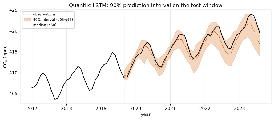
Say the number plainly: in this run the 90% interval catches 44 of 48 test months — 91.7% empirical coverage against a nominal 90%. That is a calibrated interval, and it was not guaranteed: quantile regression aims at calibration but nothing enforces it out of sample, which is why you compute coverage instead of asserting it. Two honest caveats. First, 48 consecutive months from a single forecast origin are strongly correlated, so this coverage estimate is itself noisy — a different test window could easily return 80% or 100%. Second, look at the printed widths: the interval grows from about 2.3 ppm at one month to about 6.3 ppm at four years. The model learned from the training windows that uncertainty compounds with lead time; nobody told it.
CRPS. Coverage checks one interval at one level. The continuous ranked probability score (CRPS) — the standard scoring rule of forecast verification, the number atmospheric ensemble systems report — scores the entire predictive distribution against the outcome :
It has the units of the data (ppm here), and for a forecast collapsed to a single point it reduces exactly to the absolute error — so mean CRPS is directly comparable to a point forecast’s MAE, and it rewards both calibration and sharpness at once. The second identity is also the estimator: average the pinball loss over a dense quantile grid and double it. We already predict 19 quantiles, so the implementation is a few lines.
def crps_from_quantiles(y_true, q_pred, quantiles):
    """Quantile-based CRPS estimator: 2 x the pinball loss averaged over a
    dense quantile grid. Exact in the limit of a dense grid; with 19 levels
    it slightly undervalues the tails beyond q05/q95."""
    yv = np.asarray(y_true, dtype=float).reshape(-1, 1)
    diff = yv - np.asarray(q_pred, dtype=float)
    tau = np.asarray(quantiles, dtype=float).reshape(1, -1)
    return 2.0 * np.maximum(tau * diff, (tau - 1.0) * diff).mean(axis=1)

crps_q = crps_from_quantiles(test_co2.values, q_pred, QUANTILES)
print(f"mean CRPS, quantile LSTM       : {crps_q.mean():.3f} ppm")
print(f"MAE of its median (q50)        : {np.mean(np.abs(test_co2.values - med)):.3f} ppm")
print("point forecasts (CRPS = MAE):")
for name in ["LSTM", "SARIMA"]:
    print(f"  {name:12s}: {results_co2[name]['MAE']:.3f} ppm")
mean CRPS, quantile LSTM : 0.766 ppm
MAE of its median (q50) : 1.050 ppm
point forecasts (CRPS = MAE):
LSTM : 0.886 ppm
SARIMA : 0.281 ppm
Read the three numbers together. The quantile LSTM’s mean CRPS (0.766 ppm) beats the MAE of its own median forecast (1.051 ppm) and of the point-forecast LSTM from 3.4 (0.886 ppm): spreading probability over the range where the outcome may fall earns real score even when the center is imperfect. That comparison is the entire argument for probabilistic forecasting, in one line of output. But SARIMA’s point forecast still wins at 0.281 ppm — a well-placed point beats an honestly wide distribution. Calibration does not excuse a biased or diffuse center; the verification community’s slogan is sharpness subject to calibration, and the natural next contestant would be SARIMA’s own forecast distribution (get_forecast(...).conf_int() gives its intervals — try scoring them).
3.8 Error vs lead time: the skill horizon
A single 48-month MAE flattens an entire dimension of forecast quality: how fast skill decays with lead time. Atmospheric verification never reports one number; it reports error as a function of lead, because a model that is excellent at 1 month and useless at 12 serves different decisions than one that is mediocre everywhere.
We measure it with a rolling-origin evaluation, the way operational systems are scored. The models stay frozen exactly as trained on data through 2019-08 — no retraining. The forecast origin then slides month by month through the test window; at each origin the model sees the observed history up to that month (an operational forecaster always has the latest observations) and issues forecasts for leads 1 through 12. Averaging the absolute error at each lead over all origins gives an error-vs-lead-time curve — with 37 origins per lead rather than the single sample per lead that one 48-month forecast provides.
The vocabulary to take away: the skill horizon is the lead time beyond which a model stops beating the reference forecast (persistence, here). Beyond it, the model adds nothing over “no change”. Weather models hit their skill horizon around two weeks; the question is where these models hit theirs on CO2.
LEADS = 12
LAGS_CO2, ROLL_CO2 = [1, 2, 3, 6, 12, 24], 12
y_vals = y.to_numpy()
first_test = len(train_co2)
origins = np.arange(first_test - 1, len(y) - LEADS)  # index of the last observed month

# One LightGBM fit on the training series only, reused frozen at every origin.
X_tr_lead, y_tr_lead = build_training_table(train_co2, LAGS_CO2, ROLL_CO2)
lgbm_frozen = LGBMRegressor(n_estimators=300, learning_rate=0.05, num_leaves=15,
                            random_state=0, verbose=-1).fit(X_tr_lead, y_tr_lead)

abs_err = {name: np.zeros((len(origins), LEADS))
           for name in ["naive", "seasonal naive", "LightGBM", "LSTM"]}
for r, j in enumerate(origins):
    hist = y_vals[:j + 1]                        # everything observed at the origin
    target = y_vals[j + 1:j + 1 + LEADS]
    abs_err["naive"][r] = np.abs(target - hist[-1])
    abs_err["seasonal naive"][r] = np.abs(target - y_vals[j + 1 - 12:j + 1 + LEADS - 12])
    h = list(hist)                               # LightGBM: recursive from observed history
    for step in range(LEADS):
        row = pd.DataFrame([lag_feature_row(np.asarray(h), y.index[j + 1 + step],
                                            LAGS_CO2, ROLL_CO2)])
        h.append(h[-1] + float(lgbm_frozen.predict(row)[0]))
    abs_err["LightGBM"][r] = np.abs(target - np.asarray(h[-LEADS:]))
    abs_err["LSTM"][r] = np.abs(target - nn_forecast(lstm_co2, hist[-CONTEXT_CO2:],
                                                     scale_co2)[:LEADS])

leads = np.arange(1, LEADS + 1)
lead_mae = pd.DataFrame({name: e.mean(axis=0) for name, e in abs_err.items()},
                        index=leads)
naive_train_mae_co2 = np.mean(np.abs(np.diff(train_co2.values)))

fig, ax = plt.subplots(figsize=(7, 3.5))
for name in lead_mae.columns:
    ax.plot(leads, lead_mae[name], color=COLORS[name], lw=1.5, marker="o",
            ms=3, label=name)
sec = ax.secondary_yaxis("right", functions=(lambda v: v / naive_train_mae_co2,
                                             lambda v: v * naive_train_mae_co2))
sec.set_ylabel("MASE")
ax.set_xlabel("lead time (months)")
ax.set_ylabel("MAE (ppm)")
ax.set_title(f"Error vs lead time, {len(origins)} rolling origins in the test window")
ax.legend(fontsize=8)
fig.tight_layout()
plt.show()

for name in ["seasonal naive", "LightGBM", "LSTM"]:
    wins = leads[lead_mae[name].values < lead_mae["naive"].values]
    print(f"{name:15s} beats persistence at leads: {wins.tolist()}")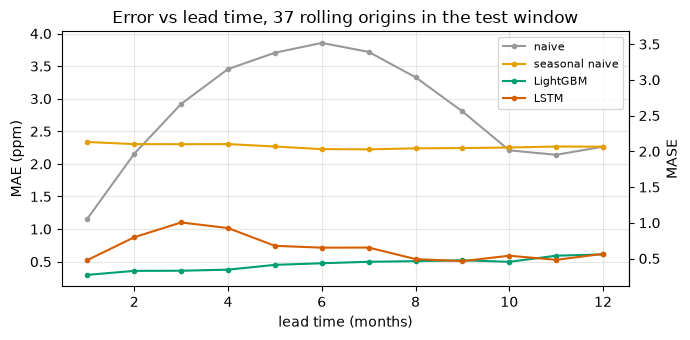
seasonal naive  beats persistence at leads: [3, 4, 5, 6, 7, 8, 9]
LightGBM        beats persistence at leads: [1, 2, 3, 4, 5, 6, 7, 8, 9, 10, 11, 12]
LSTM            beats persistence at leads: [1, 2, 3, 4, 5, 6, 7, 8, 9, 10, 11, 12]
The curve and the printed check answer the skill-horizon question, and on CO2 the answer is the opposite of weather. Persistence degrades steadily with lead — the trend and the seasonal cycle pull the series ever further from “no change” — while the trained models’ error grows far more slowly. LightGBM and the LSTM beat persistence at every lead from 1 to 12 months: their skill horizon lies beyond a year, past the longest lead we measured. Weather models lose to climatology in about two weeks because atmospheric chaos destroys the information in the initial state; monthly CO2 keeps its skill because the structure that carries the forecast (trend plus annual cycle) never stops applying. The skill horizon is a property of the series as much as of the model.
The reference forecasts are still instructive. Seasonal naive beats persistence only at intermediate leads (3 through 9 in this run): at leads 1-2 last month’s value is simply very close to the truth, and near lead 12 persistence lands back in the same season, closing most of the gap. So even the choice of reference depends on lead time — one more reason a single-number summary of forecast skill hides more than it shows. For a series where the skill horizon arrives almost immediately, run this same rolling-origin evaluation on the Jakobshavn series of Section 4.
3.9 Is the ranking stable? Seed spread
Section 4 will warn that rankings from short series are unstable across random seeds. The same admission applies right here, so we quantify it instead of leaving it as a caveat. Every number in the 3.6 table came from one training run; a table entry is a sample from a distribution over seeds, and reporting a sample as if it were the mean is the same sin as reporting a point forecast without an interval.
The seed sensitivity differs by model class, and that is part of the lesson:
- naive, seasonal naive, SARIMA are deterministic: no seed, no spread.
- LightGBM takes a
random_state, but as configured here (no row or feature subsampling) the algorithm is deterministic too — the seed is an inert knob until you enable bagging. We run 5 seeds to demonstrate that, not to estimate a spread. - LSTM and transformer are stochastic twice over: weight initialization and batch shuffling (plus dropout, for the transformer). These are the entries whose table position you should distrust from a single run. They are also the slow entries, so we use 3 seeds each rather than 5 and say so.
def mase_of(pred):
    return forecast_metrics(test_co2.values, pred, train_co2.values)["MASE"]

seed_mase = {}
seed_mase["LightGBM"] = [
    mase_of(lgbm_recursive_forecast(train_co2, test_co2.index,
                                    lags=[1, 2, 3, 6, 12, 24], roll=12,
                                    random_state=s)[0])
    for s in range(5)
]

def deep_seed_mase(model_cls, seed):
    torch.manual_seed(seed)
    m = model_cls(horizon=H_CO2)
    train_forecaster(m, Xc, Yc, epochs=40)
    return mase_of(nn_forecast(m, train_co2.to_numpy()[-CONTEXT_CO2:], scale_co2))

# Seed 0 is the run already in the 3.6 table; two more per deep model. Three
# seeds, not five: these are the slow entries, and the spread they show is
# already unmistakable.
seed_mase["LSTM"] = ([results_co2["LSTM"]["MASE"]]
                     + [deep_seed_mase(LSTMForecaster, s) for s in (1, 2)])
seed_mase["Transformer"] = ([results_co2["Transformer"]["MASE"]]
                            + [deep_seed_mase(TransformerForecaster, s) for s in (1, 2)])

spread_table = pd.DataFrame({
    name: {"MASE mean": np.mean(v), "MASE std": np.std(v),
           "MASE min": np.min(v), "MASE max": np.max(v), "seeds": len(v)}
    for name, v in seed_mase.items()}).T.round(3)
spread_tableThe spread table sharpens the 3.6 ranking rather than overturning it — and shows exactly where the randomness lives:
- LightGBM posts the identical MASE for all five seeds (std 0.000), as promised: with no row or feature subsampling the algorithm is deterministic, and “we varied the seed” is evidence of robustness only when the algorithm actually consumes the seed.
- LSTM spans 0.808-0.856 (mean 0.827, std 0.021); the transformer spans 0.327-0.403 (mean 0.356, std 0.034) — a tenth of its own mean, from initialization, batch order, and dropout alone.
- The ranges do not overlap each other, SARIMA’s deterministic 0.256, or LightGBM’s 0.939, so on this run the shootout order survives the seeds. That is a conclusion we can now state with evidence instead of hope — and it is not a general law. On the ice series below, the gaps between models are of the same size as spreads like these, which is why its ranking should not be trusted from a single run. Report mean and spread; let the reader see whether the gaps beat the noise.
4. The ice series: a harder test
We run the ice series through the baselines, ARIMA, LightGBM, and the LSTM only. Fewer models on purpose: the series is short (about 350 training samples), irregularly sampled, and not dominated by a clean seasonal cycle, so a seasonal SARIMA has little to grab onto and a transformer has too little data to earn its parameters. Adding them would pad the table, not the insight.
4.1 Baselines and ARIMA
The sampling averages about 46 samples per year, so the “seasonal naive” tiles the last 46 training samples as an approximate last-year copy; with irregular sampling this alignment is only approximate, one more reason seasonal machinery helps less here. For the classical entry we use a plain ARIMA(1,1,1), no seasonal terms.
from statsmodels.tsa.arima.model import ARIMA

H_ICE = len(test_ice)
m_ice = 46   # approx. one year (~46 samples/yr on average)

naive_ice = np.full(H_ICE, train_ice.iloc[-1])
seasonal_ice = np.tile(train_ice.values[-m_ice:],
                       int(np.ceil(H_ICE / m_ice)))[:H_ICE]

register(results_ice, preds_ice, "naive", naive_ice, test_ice, train_ice)
register(results_ice, preds_ice, "seasonal naive", seasonal_ice, test_ice, train_ice)

with warnings.catch_warnings():
    warnings.simplefilter("ignore")
    arima_ice = ARIMA(train_ice.values, order=(1, 1, 1)).fit()
register(results_ice, preds_ice, "ARIMA", arima_ice.forecast(H_ICE), test_ice, train_ice)
naive -> {'MSE': np.float64(34556.717), 'RMSE': np.float64(185.894), 'MAE': np.float64(168.382), 'MAPE (%)': np.float64(9.589), 'MASE': np.float64(6.249)}
seasonal naive -> {'MSE': np.float64(23662.811), 'RMSE': np.float64(153.827), 'MAE': np.float64(129.081), 'MAPE (%)': np.float64(7.237), 'MASE': np.float64(4.79)}
ARIMA -> {'MSE': np.float64(32800.223), 'RMSE': np.float64(181.108), 'MAE': np.float64(163.157), 'MAPE (%)': np.float64(9.297), 'MASE': np.float64(6.055)}
4.2 LightGBM and the LSTM, reused
Same helpers, new lag sets: lags up to 46 samples (about a year) and a short rolling mean. The LSTM uses a roughly one-year context (46 samples) and forecasts the whole test window directly, as before.
lgbm_pred_ice, _ = lgbm_recursive_forecast(train_ice, test_ice.index,
                                           lags=[1, 2, 3, 6, 23, 46], roll=6)
register(results_ice, preds_ice, "LightGBM", lgbm_pred_ice, test_ice, train_ice)
LightGBM -> {'MSE': np.float64(13027.719), 'RMSE': np.float64(114.139), 'MAE': np.float64(94.373), 'MAPE (%)': np.float64(5.338), 'MASE': np.float64(3.502)}
CONTEXT_ICE = 46
Xi, Yi = make_windows(train_ice.to_numpy(), CONTEXT_ICE, H_ICE)
scale_ice = float(Xi.std())
Xi, Yi = Xi / scale_ice, Yi / scale_ice
print(f"{len(Xi)} training windows, scale = {scale_ice:.0f} m/yr")

torch.manual_seed(0)
lstm_ice = LSTMForecaster(horizon=H_ICE)
_ = train_forecaster(lstm_ice, Xi, Yi, epochs=40)
lstm_pred_ice = nn_forecast(lstm_ice, train_ice.to_numpy()[-CONTEXT_ICE:], scale_ice)
register(results_ice, preds_ice, "LSTM", lstm_pred_ice, test_ice, train_ice)
213 training windows, scale = 83 m/yr
LSTM -> {'MSE': np.float64(62535.969), 'RMSE': np.float64(250.072), 'MAE': np.float64(218.994), 'MAPE (%)': np.float64(12.499), 'MASE': np.float64(8.127)}
ice_table = pd.DataFrame(results_ice).T.sort_values("MASE").round(3)
ice_tablefig, ax = plt.subplots(figsize=(9, 4))
recent_ice = ice.loc["2020":]
ax.plot(recent_ice.index, recent_ice.values, color=COLORS["observations"],
lw=1.5, label="observations")
for name, pred in preds_ice.items():
ax.plot(test_ice.index, pred, color=COLORS[name], lw=1.2, ls="--", label=name)
ax.axvline(test_ice.index[0], color="0.6", lw=0.8)
ax.set_xlabel("year")
ax.set_ylabel("surface speed (m/yr)")
ax.set_title("Ice test window: all forecasts vs observations")
ax.legend(fontsize=8, ncol=2)
fig.tight_layout()
plt.show()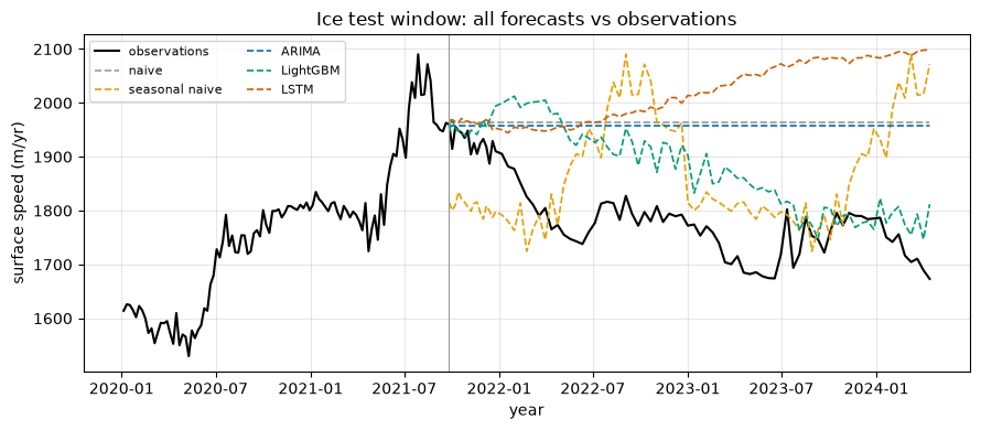
Note how much larger the MASE values are than for CO2, across every model. The one-step naive game (the MASE denominator) is easy on a slowly varying speed series, but the multi-year test window contains changes in glacier behavior that no pattern in the training window announces. When the future is not written in the past, more model does not mean more forecast. Also expect the ranking among the trained models to be unstable here: with ~340 training samples, small choices (context length, lag set, random seed) move models up and down the table — we measured exactly this effect on the CO2 shootout in Section 3.9, and it is worse on a series this short. Report that honestly rather than shopping for the settings that look best.
5. Rare events break bulk metrics
The defining data problem of the geosciences is a field that varies smoothly for years and then does something extreme for three days: floods on a discharge record, eruptions on a tremor record, offsets on a strain record. Every metric in this notebook so far averages over all test samples, and quiet samples outnumber event samples by roughly twelve to one — so a model can post an excellent MAE while missing every event that matters.
To show this cleanly we need ground truth about the events, so we build the series ourselves with mlgeo_synth.inject_rare_events: eight years of a daily seasonal background, punctuated by ~6 events per year lasting 2-6 days, with amplitudes drawn from a generalized Pareto distribution (tail="gpd", shape ). That is a power-law tail — the extreme-value regime of real flood and surge records, where the variance is infinite and the largest event in any future window is routinely several times larger than the largest one yet observed. The generator returns an amplitude column: the true drawn size of each event, exactly the ground truth a bulk metric never sees.
The forecaster is deliberately given every advantage: one-step-ahead LightGBM (yesterday’s value is always in the feature set), trained on six years, tested on the last two. Then, instead of one MAE, we stratify the test error by the ground-truth amplitude.
n_days_ev = int(8 * 365.25)
days_ev = pd.date_range("2015-01-01", periods=n_days_ev, freq="D")
rng_ev = np.random.default_rng(0)
background_ev = (10.0 + 3.0 * np.sin(2 * np.pi * np.arange(n_days_ev) / 365.25)
                 + 0.3 * rng_ev.standard_normal(n_days_ev))
events = mlgeo_synth.inject_rare_events(background_ev, rate_per_year=6.0,
                                        duration_days=(2, 6), shape="spike",
                                        tail="gpd", seed=7)
series_ev = pd.Series(events["value"].to_numpy(), index=days_ev)

# One-step-ahead LightGBM on lag features — the easiest possible forecasting
# task: the model always has yesterday's observation in hand.
LAGS_EV, ROLL_EV = [1, 2, 3, 5, 7, 14, 365], 7
X_ev, dy_ev = build_training_table(series_ev, LAGS_EV, ROLL_EV)
start_ev = max(max(LAGS_EV), ROLL_EV)
dates_ev = series_ev.index[start_ev:]
cut = dates_ev.searchsorted(pd.Timestamp("2021-01-01"))   # train < 2021 <= test

lgbm_ev = LGBMRegressor(n_estimators=300, learning_rate=0.05, num_leaves=15,
                        random_state=0, verbose=-1).fit(X_ev.iloc[:cut], dy_ev[:cut])
pred_ev = (series_ev.to_numpy()[start_ev - 1:-1][cut:]
           + lgbm_ev.predict(X_ev.iloc[cut:]))            # previous value + predicted change
true_ev = series_ev.to_numpy()[start_ev:][cut:]
err_ev = np.abs(true_ev - pred_ev)

# Stratify by the generator's ground-truth amplitude column.
evt = events.iloc[start_ev:].iloc[cut:]                   # aligned truth columns
quiet = evt["event"].to_numpy() == 0
amp = evt["amplitude"].to_numpy()
strata = {
    "all test samples":        np.ones_like(quiet),
    "quiet (no event)":        quiet,
    "event, amplitude < 10":   ~quiet & (amp < 10),
    "event, amplitude 10-25":  ~quiet & (amp >= 10) & (amp < 25),
    "event, amplitude >= 25":  ~quiet & (amp >= 25),
}
tail_table = pd.DataFrame({name: {"n samples": int(m.sum()),
                                  "MAE": err_ev[m].mean()}
                           for name, m in strata.items()}).T
tail_table["n samples"] = tail_table["n samples"].astype(int)
print(tail_table.round(3))
print(f"\nlargest single miss: {err_ev.max():.1f} "
      f"(event amplitude {amp[np.argmax(err_ev)]:.1f})")

# Left: the test window. Right: per-event peak error vs true amplitude.
per_event = (pd.DataFrame({"event_id": evt["event_id"].to_numpy(),
                           "amp": amp, "err": err_ev})
             .query("event_id >= 0").groupby("event_id")
             .agg(amp=("amp", "max"), peak_err=("err", "max")))
fig, axes = plt.subplots(1, 2, figsize=(10, 3.5),
                         gridspec_kw={"width_ratios": [2, 1]})
axes[0].plot(dates_ev[cut:], true_ev, color=COLORS["observations"], lw=0.8,
             label="observed")
axes[0].plot(dates_ev[cut:], pred_ev, color=COLORS["LightGBM"], lw=0.8,
             alpha=0.8, label="one-step forecast")
axes[0].set_ylabel("value")
axes[0].set_title("Test window (events ride on the seasonal background)")
axes[0].legend(fontsize=8)
axes[1].loglog(per_event["amp"], per_event["peak_err"], "o", ms=5,
               color=COLORS["LightGBM"])
lim = [4, per_event["amp"].max() * 1.5]
axes[1].plot(lim, lim, color="0.6", lw=0.8, ls="--", label="error = amplitude")
axes[1].set_xlabel("true event amplitude")
axes[1].set_ylabel("peak |error| in event")
axes[1].set_title("Misses scale with amplitude")
axes[1].legend(fontsize=8)
fig.tight_layout()
plt.show()
n samples MAE
all test samples 730 0.969
quiet (no event) 674 0.621
event, amplitude < 10 43 2.458
event, amplitude 10-25 7 10.577
event, amplitude >= 25 6 18.274
largest single miss: 50.8 (event amplitude 50.2)
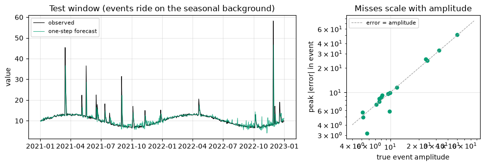
A naive reading of the first row says the model is excellent: MAE 0.97 on a series whose seasonal swing alone is 6 units. The stratified rows tell the real story. Quiet days score 0.62 — the noise floor, as good as one-step forecasting gets. Small events (amplitude below 10) already cost 2.5. The seven samples in mid-size events cost about 10.6, the six samples in the largest events 18.3, and the single largest event — amplitude 50.2 — is missed by 50.8: the model predicted the seasonal background and the flood happened anyway. The right panel makes it systematic: peak error per event tracks the true amplitude along the error-equals-amplitude line. What the model has never seen, it misses in full.
Both causes are structural, not bugs. Event onsets are unpredictable from lag features — no yesterday-value tells you a spike starts tomorrow — and the GPD tail () guarantees that the test window contains amplitudes beyond every training example, so the model is extrapolating precisely on the samples that matter most. Meanwhile the bulk metric hides all of it: event samples are 56 of 730 test days (about one in thirteen), so the overall MAE (0.97) sits within a factor of 1.6 of the quiet-day floor while the top stratum is thirty times worse. A leaderboard scored on overall MAE would congratulate this model.
The repair is in the metric, not the model: if events are what your forecast exists for — floods, eruptions, offsets — score them separately. Stratified tables like this one, event-window recall, or amplitude-weighted losses all work; averaging over the quiet days does not. This is the same fair-evaluation discipline as the hidden leaderboard track below: what you measure is what you optimize, so measure the thing that matters.
6. Exercises
Exercise 1. In the CO2 LightGBM entry, remove lag_12 and lag_24 from the lag list and rerun. What happens to the MASE, and why?
Solution
The MASE gets worse. The 12- and 24-month lags are how the model sees the annual cycle; without them it must reconstruct seasonality from the calendar-month feature and short lags alone, and the recursive forecast slowly drifts off the seasonal shape. Run
lgbm_recursive_forecast(train_co2, test_co2.index, lags=[1, 2, 3, 6], roll=12)
and compare the metrics with forecast_metrics.
Exercise 2. The deep models forecast all 48 months in one shot (direct multi-step); LightGBM predicts one month at a time and feeds predictions back in (recursive). Name one advantage of each strategy.
Solution
Direct: no error feedback, so a bad early step cannot contaminate later steps, and the model is trained on exactly the horizon it is scored on. Recursive: one model serves any horizon, and one-step training uses many more examples per parameter; but errors compound along the horizon. Hybrids (one direct model per step, or “rectify” schemes) exist for exactly this trade-off.
Exercise 3. Rerun Section 5 twice: once with tail="uniform" (the generator’s default: amplitudes uniform on 5-20) and once keeping tail="gpd" but raising rate_per_year to 24. Which change does more for the large-event stratum, and what does that tell you about the difference between rare and heavy-tailed?
Solution
The uniform tail helps more. With amplitudes capped at 20, the training window has already shown the model events as large as any it will ever be scored on — the problem is interpolation, and more examples (higher rate) polish it. With a GPD tail the largest future event is beyond every training example almost by construction, so no realistic event rate fixes the top stratum: the model is asked to extrapolate. Rarity limits how many examples you get; a heavy tail guarantees the exam contains a magnitude the textbook never showed. (Chapter 4.5’s out-of-distribution exercise is the same lesson in feature space.)
7. The class leaderboard: two tracks
Now the 12 months we removed in Section 1.2 come back into play — but first, an honest disclosure about what a public leaderboard can and cannot measure.
Track A — CO2 (diagnostic).
- Produce a 12-month CO2 forecast for 2023-09 through 2024-08, the held-out months, using any model trained on data up to 2023-08 only. On your honor — see the box above for why cheating here only defeats the diagnostic.
- Save it to
results/forecast_<uwnetid>.csvwith exactly two columns:date(asYYYY-MM) andco2_ppm. - Submit it via a pull request to the course book repository, https://
github .com /geo -smart /mlgeo -book. CI scores each PR and posts the standings.
Scoring is MASE against the held-out months, scaled by the naive one-step MAE of the training series (the same convention as forecast_metrics in Section 2.2 — the denominator comes from the pre-holdout record, not from the holdout itself).
Track B — the hidden synthetic series (graded). The file leaderboard/synth_forecast_history.csv in the course repository holds a daily displacement series from mlgeo_synth.gnss_series — secular trend, annual and semi-annual cycles, and colored noise, like the GNSS records of Chapter 2 — generated from a private seed and regenerated every year. Forecast the 90 days after the last history date and save results/forecast_hidden_<uwnetid>.csv with columns date (YYYY-MM-DD) and disp_mm, submitted in the same pull request. The truth series is never committed; the public leaderboard lists your submission as received, and the instructor’s run produces the scored table. Same metric: MASE, scaled by the history’s naive one-step error.
The cells below write an example file for each track using the recursive LightGBM model. Replace example with your UW NetID and the forecasts with your own.
uwnetid = "example"   # <-- replace with your UW NetID

# Track A: refit on ALL pre-holdout data (through 2023-08) and forecast the
# 12 holdout months.
final_pred, _ = lgbm_recursive_forecast(y, holdout_months,
                                        lags=[1, 2, 3, 6, 12, 24], roll=12)

submission = pd.DataFrame({"date": holdout_months.strftime("%Y-%m"),
                           "co2_ppm": np.round(final_pred, 2)})
os.makedirs("results", exist_ok=True)
out_path = f"results/forecast_{uwnetid}.csv"
submission.to_csv(out_path, index=False)
print("wrote", out_path)
print(submission.to_string(index=False))
wrote results/forecast_example.csv
date co2_ppm
2023-09 418.23
2023-10 418.42
2023-11 419.86
2023-12 421.29
2024-01 422.44
2024-02 423.25
2024-03 424.07
2024-04 425.49
2024-05 426.23
2024-06 425.65
2024-07 423.90
2024-08 421.89
# Track B: forecast the hidden synthetic series 90 days past its history.
hist_path = Path("../../leaderboard/synth_forecast_history.csv")
if not hist_path.exists():          # running outside the repo checkout
    hist_path = Path(pooch.retrieve(
        "https://raw.githubusercontent.com/geo-smart/mlgeo-book/main/"
        "leaderboard/synth_forecast_history.csv",
        known_hash=None, fname="synth_forecast_history.csv"))
hidden_hist = pd.read_csv(hist_path, parse_dates=["date"])
hidden_series = pd.Series(hidden_hist["disp_mm"].to_numpy(),
                          index=pd.DatetimeIndex(hidden_hist["date"]))
horizon_dates = pd.date_range(hidden_series.index[-1] + pd.Timedelta(days=1),
                              periods=90, freq="D")
print(f"history: {len(hidden_series)} days ending {hidden_series.index[-1].date()}; "
      f"forecast {horizon_dates[0].date()} .. {horizon_dates[-1].date()}")

hidden_pred, _ = lgbm_recursive_forecast(hidden_series, horizon_dates,
                                         lags=[1, 2, 3, 7, 14, 365], roll=7)
hidden_sub = pd.DataFrame({"date": horizon_dates.strftime("%Y-%m-%d"),
                           "disp_mm": np.round(hidden_pred, 3)})
hidden_out = f"results/forecast_hidden_{uwnetid}.csv"
hidden_sub.to_csv(hidden_out, index=False)
print("wrote", hidden_out)
hidden_sub.head()
history: 2832 days ending 2022-10-02; forecast 2022-10-03 .. 2022-12-31
wrote results/forecast_hidden_example.csv
Summary
- Baselines first: naive and seasonal-naive forecasts set the bar, and MASE measures every model against the naive one-step game.
- One temporal split, one metric helper, one programmatic table. Random splits and hand-typed numbers are how the 2024 edition went wrong; do not repeat either.
- On long, structured series (CO2), a well-chosen classical model (SARIMA) is hard to beat, and deep models need care (anchoring, scaling) just to compete. On short, irregular series (Jakobshavn), every model struggles, and saying so is the correct result.
- Recursive vs direct multi-step forecasting is a real design choice; we used recursive for LightGBM and direct for the LSTM and transformer.
- A point forecast is the start, not the end. A quantile head trained on the pinball loss produced a 90% interval whose empirical coverage we measured instead of assumed, and CRPS — verification’s generalization of MAE — scored the whole distribution.
- Error is a function of lead time; plot it. The skill horizon — the lead at which a model stops beating persistence — is the operational summary of a forecast system.
- A ranking from one seed is one sample. The deterministic entries (baselines, SARIMA, this LightGBM configuration) have zero spread; the deep entries move enough across seeds to swap places. Report mean and spread, not a single draw.
- Bulk MAE can look excellent while every large rare event is missed: with heavy-tailed (GPD) amplitudes, the top event stratum carried errors thirty times the quiet-day MAE, and the largest event was missed almost in full. Stratify your scoring, or your metric will hide exactly the samples that matter.
- The leaderboard has two tracks because its public holdout is public data: the CO2 score is a diagnostic (and trivially gameable — we say so in print), while the hidden synthetic series, regenerated yearly from a private seed, carries the grading weight.
Next: submit your two leaderboard forecasts, then continue to the final project assignment (4.20). For the sequence architectures themselves, look back at notebook 4.4; for the boosting machinery, Chapter 3.