Convolutional neural networks (CNNs) are the workhorse of deep learning on structured data: images, spectrograms, and time series. This notebook covers:
- Convolutions and kernels, applied by hand to an image.
- The building blocks of a CNN: convolution, activation, pooling, fully connected layers.
- LeNet-5 on MNIST digits, written in PyTorch — the warm-up.
- A 2-D CNN regressing warming trends from a gridded synthetic climate field, against a least-squares baseline.
- A 1-D CNN earthquake detector trained on synthetic seismograms, its detection floor as a function of signal-to-noise ratio, and the classical STA/LTA detector measured on the same traces.
- A reality check: the synthetic-trained detector scored on real, labeled miniPNW waveforms.
- How to translate a published architecture table into working code.
import os

import numpy as np
import matplotlib.pyplot as plt
import torch
import torch.nn as nn
import torchinfo
from scipy.signal import convolve2d
from skimage import data

# Device-agnostic setup: CUDA GPU, Apple silicon (MPS), or CPU.
device = torch.device("cuda" if torch.cuda.is_available()
                      else "mps" if torch.backends.mps.is_available()
                      else "cpu")
print(f"Using device: {device}")
Using device: cpu
0. To review
At this point, you should understand:
- The perceptron
- The role of activation functions
- Why and how to implement a simple gradient descent
- Loss functions
- Batching
- Multilayer perceptrons
1. Convolutions
Just like perceptrons and multilayer perceptrons, each element in a CNN receives inputs, performs a dot product, and passes that product through an activation function. The difference is that a CNN applies the same small set of weights, called a kernel, everywhere in the input. These networks work well on structured 1-D, 2-D, and 3-D data such as time series and images.
As their name implies, CNNs rely on convolutions:
where is the input, is the kernel of convolution, and τ is a dummy variable.
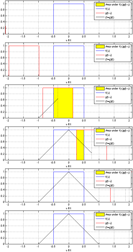
For discrete functions, you simply sum:
Convolution extends to multiple dimensions.
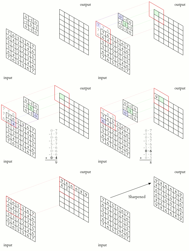
For example, consider the mean filter (here, for a 3 x 3 kernel):
# Load an example image from scikit-image
image = data.coins()

# Kernel size
filterDimension = 3

# Define a mean filter
mean_filter = np.ones((filterDimension, filterDimension)) / (filterDimension * filterDimension)

# Apply the mean filter to the image using convolution
filtered_image = convolve2d(image, mean_filter, mode='same', boundary='symm')

fig, ax = plt.subplots(1, 2, figsize=(8, 3))
ax[0].imshow(image, cmap='gray')
ax[0].set_title('Original image')
ax[1].imshow(filtered_image, cmap='gray')
ax[1].set_title('Mean-filtered image')
for a in ax:
    a.axis('off')
fig.tight_layout()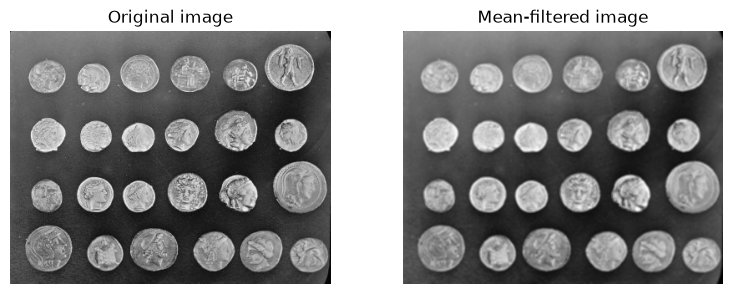
The mean filter blurs. Other kernels detect structure. The Sobel filters approximate the image gradient and respond to edges:
# Sobel filters
sobel_filter_horizontal = np.array([
    [-1, -2, -1],
    [0, 0, 0],
    [1, 2, 1]
])

sobel_filter_vertical = np.array([
    [-1, 0, 1],
    [-2, 0, 2],
    [-1, 0, 1]
])

# Apply the Sobel filters to the image
result_horizontal = convolve2d(image, sobel_filter_horizontal)
result_vertical = convolve2d(image, sobel_filter_vertical)

# Combine the horizontal and vertical edges to get the overall edges
edges = np.sqrt(result_horizontal**2 + result_vertical**2)

# Thresholding to accentuate the edges
threshold = 10
edges[edges < threshold] = 0

fig, axes = plt.subplots(1, 4, figsize=(13, 3.2))
axes[0].imshow(image, cmap='gray')
axes[0].set_title('Original image')
axes[1].imshow(result_horizontal, cmap='gray')
axes[1].set_title('Horizontal Sobel')
axes[2].imshow(result_vertical, cmap='gray')
axes[2].set_title('Vertical Sobel')
axes[3].imshow(edges, cmap='gray')
axes[3].set_title('Combined edges (thresholded)')
for a in axes:
    a.axis('off')
fig.tight_layout()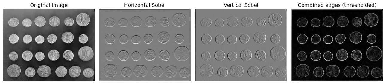
The point of a CNN is that it does not use hand-designed kernels like these. It learns the kernel weights from data by gradient descent. Early layers often end up learning edge detectors on their own.
Exercise 1. Change filterDimension from 3 to 15 in the mean-filter cell. What happens to the coins, and why?
Solution
A 15 x 15 mean filter averages over a much larger neighborhood, so the image becomes strongly blurred and small features (the texture inside the coins, the gaps between them) disappear. The kernel size sets the spatial scale of the features a convolution responds to.
2. Assembling a CNN
The architecture of a CNN classically comprises:
- A convolutional layer
- An activation layer
- A pooling layer
- A fully connected layer
2.1 The convolutional layer
Here we consider a CNN that takes in images and returns some output.
Aspects of this layer:
Inputs: In the case of 2D convolutions, three dimensions: height, width, depth.
Filters: The convolutional kernels, each with a bias and a weight for each element of the kernel. The output of a filter is a feature map. Generally, the number of filters is greater than the input depth. The kernel size is often square, but does not need to be.
Stride: The step size by which the filter moves.
Padding: Values added to the edges of the input.
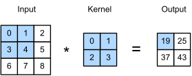
Convolution with kernel window (Fig. 7.2.1 from Dive into Deep Learning).
In the example above, the top-left output value is 0×0 + 1×1 + 3×2 + 4×3 = 19. We repeat the process until all elements of the output map are filled, and we repeat this for each filter.
A good lecture about CNNs is Stanford’s CS230 cheatsheet.
How would you interpret the following code?
# pytorch version
torch.nn.Conv2d(in_channels=3, out_channels=64, kernel_size=6)
Conv2d(3, 64, kernel_size=(6, 6), stride=(1, 1))This layer takes an input with 3 channels (for example an RGB image), applies 64 filters of size 6 x 6 (each spanning all 3 input channels), and outputs 64 feature maps.
2.2 The activation layer
The convolutional layer is followed by an activation layer. This layer applies an activation function, such as ReLU (Rectified Linear Unit), to the outputs of the convolution.
# Define the ReLU function
def relu(x):
    return np.maximum(0, x)

x = np.linspace(-5, 5, 100)
y_relu = relu(x)

fig, ax = plt.subplots(figsize=(5, 3.5))
ax.plot(x, y_relu, label='ReLU')
ax.set_xlabel('x')
ax.set_ylabel('ReLU(x)')
ax.axhline(0, color='black', linewidth=0.5)
ax.axvline(0, color='black', linewidth=0.5)
ax.grid(color='gray', linestyle='--', linewidth=0.5)
ax.legend()
plt.show()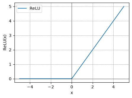
2.3 The pooling layer
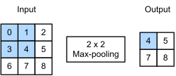
The pooling layer downsamples the feature maps. By combining values, pooling reduces the size of the model and makes it less sensitive to small shifts of the input.
Max pooling layers take the maximum value within a given neighborhood (set by the pooling size).
2.4 The fully connected layer
Finally, we include a fully connected layer (every input connected to every output). For classification, CNNs typically end with a softmax that transforms the outputs of the last fully connected layer into class probabilities (values between 0 and 1 that sum to 1).
2.5 Some notes
In the convolutional layer, the neurons are not connected to every part of the input data.
A dense layer learns global patterns. A convolution layer learns local patterns and is translation equivariant: shift the input and the feature map shifts with it, so a pattern learned in one part of the image (or time series) is detected anywhere else. The approximate translation invariance of a full CNN, the same prediction wherever the pattern sits, comes from the pooling layers that discard position as they downsample; the 1-D detector in Section 5 gets its shift tolerance from its global average pool. CNNs also learn hierarchical patterns: a first layer learns a local pattern, a second layer combines the local features into broader-scale features.
2.6 Aside: image segmentation vocabulary
Classification assigns one label to a whole image. Segmentation assigns labels at the pixel level, and comes in three flavors. A standard illustration is a street scene shown three ways: semantic segmentation colors every pixel by class (road, sky, person, car) without separating individuals; instance segmentation outlines each individual object (this person, that car) separately; panoptic segmentation combines both, labeling every pixel by class while keeping object instances distinct.
3. LeNet-5 on MNIST
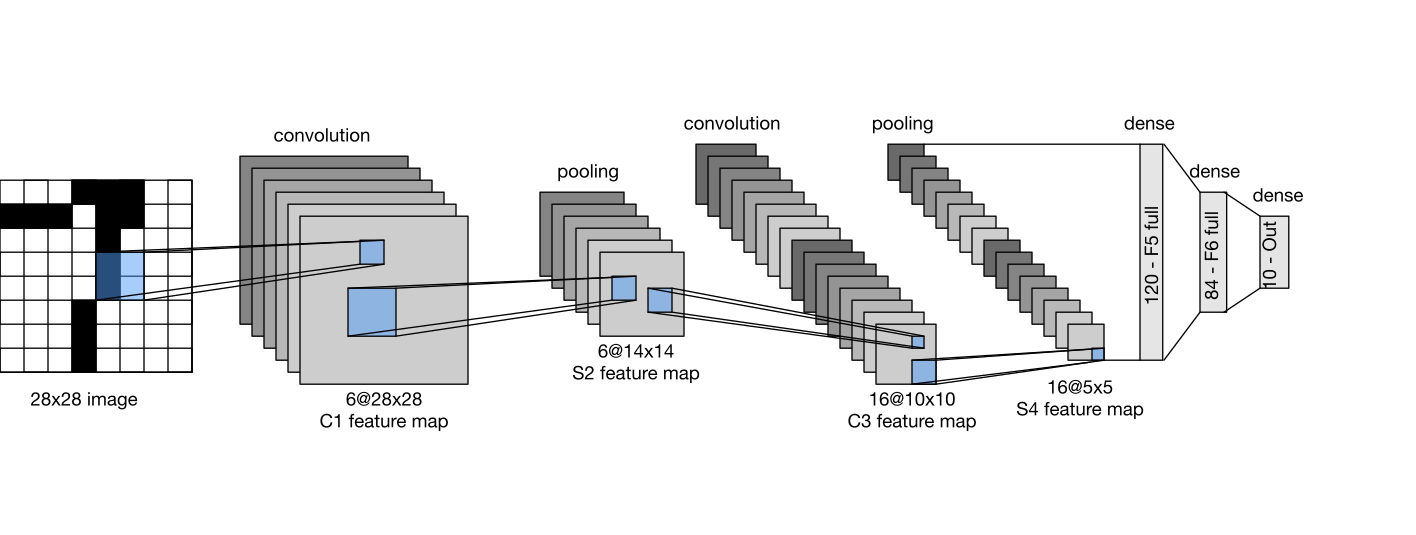
MNIST is deep learning’s hello-world: small, clean, and nothing like a geoscience dataset. We use it as the warm-up, to get the training mechanics right on a problem where nothing else can go wrong; the geoscience payload starts in Section 4. We now build the LeNet-5 architecture (LeCun et al., 1998), one of the first successful CNNs, and train it to classify handwritten digits from MNIST. The network is a sequential stack of 2 convolutional layers and 3 fully connected layers. A common graphical representation:
3.1 Load the data
We use torchvision to download MNIST. The full training set has 60,000 images; to keep this notebook fast we train on a subset of 6,000 and evaluate on 1,500 test images. On your own machine you can raise these numbers (and the number of epochs) for better accuracy.
from torch.utils.data import DataLoader, Subset, TensorDataset
from torchvision import datasets
from torchvision.transforms import Compose, Normalize, ToTensor

data_root = os.path.expanduser("~/.cache/mlgeo-mnist")
transform = Compose([ToTensor(), Normalize([0.5], [0.5])])

train_full = datasets.MNIST(root=data_root, train=True, download=True, transform=transform)
test_full = datasets.MNIST(root=data_root, train=False, download=True, transform=transform)

# Subsets for speed
train_set = Subset(train_full, range(6000))
test_set = Subset(test_full, range(1500))

loaded_train = DataLoader(train_set, batch_size=64, shuffle=True)
loaded_test = DataLoader(test_set, batch_size=256)

X, y = next(iter(loaded_train))
print("One batch of images:", X.shape, "labels:", y.shape)
0%| | 0.00/9.91M [00:00<?, ?B/s] 1%| | 98.3k/9.91M [00:00<00:10, 929kB/s] 3%|▎ | 262k/9.91M [00:00<00:07, 1.28MB/s] 6%|▌ | 590k/9.91M [00:00<00:04, 2.08MB/s] 12%|█▏ | 1.21M/9.91M [00:00<00:02, 3.53MB/s] 23%|██▎ | 2.33M/9.91M [00:00<00:01, 5.97MB/s] 45%|████▍ | 4.46M/9.91M [00:00<00:00, 10.6MB/s] 85%|████████▍ | 8.39M/9.91M [00:00<00:00, 19.0MB/s]100%|██████████| 9.91M/9.91M [00:00<00:00, 13.0MB/s]
0%| | 0.00/28.9k [00:00<?, ?B/s]100%|██████████| 28.9k/28.9k [00:00<00:00, 538kB/s]
0%| | 0.00/1.65M [00:00<?, ?B/s] 6%|▌ | 98.3k/1.65M [00:00<00:01, 925kB/s] 18%|█▊ | 295k/1.65M [00:00<00:00, 1.46MB/s] 38%|███▊ | 623k/1.65M [00:00<00:00, 2.18MB/s] 78%|███████▊ | 1.28M/1.65M [00:00<00:00, 3.73MB/s]100%|██████████| 1.65M/1.65M [00:00<00:00, 3.41MB/s]
0%| | 0.00/4.54k [00:00<?, ?B/s]100%|██████████| 4.54k/4.54k [00:00<00:00, 9.55MB/s]One batch of images: torch.Size([64, 1, 28, 28]) labels: torch.Size([64])
# Display 3 images from one batch
images, labels = next(iter(loaded_train))
fig, axes = plt.subplots(1, 3, figsize=(8, 3))
for i in range(3):
    axes[i].imshow(images[i].numpy().squeeze(), cmap='gray')
    axes[i].set_title(f"Label: {labels[i].item()}")
    axes[i].axis('off')
plt.show()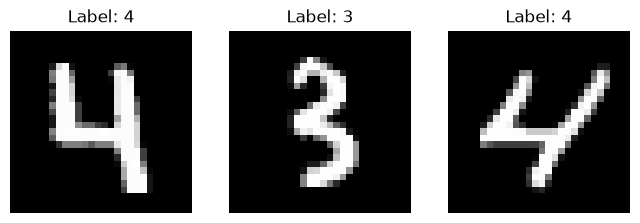
3.2 The model
We write LeNet-5 as a torch.nn.Sequential stack. The Reshape module makes sure the input is shaped (batch, channels, height, width), which is what Conv2d expects.
class Reshape(torch.nn.Module):
    def forward(self, x):
        return x.view(-1, 1, 28, 28)

model_lenet = torch.nn.Sequential(
    Reshape(),
    nn.Conv2d(1, 6, kernel_size=5, padding=2), nn.Sigmoid(),
    nn.AvgPool2d(kernel_size=2, stride=2),
    nn.Conv2d(6, 16, kernel_size=5), nn.Sigmoid(),
    nn.AvgPool2d(kernel_size=2, stride=2),
    nn.Flatten(),
    nn.Linear(16 * 5 * 5, 120), nn.Sigmoid(),
    nn.Linear(120, 84), nn.Sigmoid(),
    nn.Linear(84, 10),
)
# Walk a dummy input through the network and watch the shape change
Xd = torch.rand(size=(1, 1, 28, 28), dtype=torch.float32)
print('Initial input shape: \t', Xd.shape)
for layer in model_lenet:
Xd = layer(Xd)
print(layer.__class__.__name__, 'output shape: \t', Xd.shape)Initial input shape: torch.Size([1, 1, 28, 28])
Reshape output shape: torch.Size([1, 1, 28, 28])
Conv2d output shape: torch.Size([1, 6, 28, 28])
Sigmoid output shape: torch.Size([1, 6, 28, 28])
AvgPool2d output shape: torch.Size([1, 6, 14, 14])
Conv2d output shape: torch.Size([1, 16, 10, 10])
Sigmoid output shape: torch.Size([1, 16, 10, 10])
AvgPool2d output shape: torch.Size([1, 16, 5, 5])
Flatten output shape: torch.Size([1, 400])
Linear output shape: torch.Size([1, 120])
Sigmoid output shape: torch.Size([1, 120])
Linear output shape: torch.Size([1, 84])
Sigmoid output shape: torch.Size([1, 84])
Linear output shape: torch.Size([1, 10])
torchinfo.summary(model_lenet, input_size=(1, 1, 28, 28))==========================================================================================
Layer (type:depth-idx) Output Shape Param #
==========================================================================================
Sequential [1, 10] --
├─Reshape: 1-1 [1, 1, 28, 28] --
├─Conv2d: 1-2 [1, 6, 28, 28] 156
├─Sigmoid: 1-3 [1, 6, 28, 28] --
├─AvgPool2d: 1-4 [1, 6, 14, 14] --
├─Conv2d: 1-5 [1, 16, 10, 10] 2,416
├─Sigmoid: 1-6 [1, 16, 10, 10] --
├─AvgPool2d: 1-7 [1, 16, 5, 5] --
├─Flatten: 1-8 [1, 400] --
├─Linear: 1-9 [1, 120] 48,120
├─Sigmoid: 1-10 [1, 120] --
├─Linear: 1-11 [1, 84] 10,164
├─Sigmoid: 1-12 [1, 84] --
├─Linear: 1-13 [1, 10] 850
==========================================================================================
Total params: 61,706
Trainable params: 61,706
Non-trainable params: 0
Total mult-adds (Units.MEGABYTES): 0.42
==========================================================================================
Input size (MB): 0.00
Forward/backward pass size (MB): 0.05
Params size (MB): 0.25
Estimated Total Size (MB): 0.30
==========================================================================================3.3 Training setup
We need to choose some training parameters:
- The error metric: accuracy
- The loss function: cross-entropy for multiclass classification
- The batch size (64 here)
- The number of epochs (2 here, for speed)
- The optimizer: Adam, a variant of stochastic gradient descent that uses estimates of the first and second moments of the gradient to adapt the learning rate for each weight
The training function below is generic: it takes any model and any pair of data loaders, so we will reuse it in Section 5. It moves each batch to device, runs the forward pass, backpropagates the loss, and updates the weights. After each epoch it evaluates loss and accuracy on the validation loader (with gradients turned off).
The function also keeps a checkpoint: a copy of the weights from the epoch with the best validation accuracy, restored at the end. Stochastic training does not improve monotonically, so the last epoch is not always the best one. In production you would write the checkpoint to disk with torch.save({'state_dict': model.state_dict()}, 'checkpoint.pt'); here we keep it in memory.
def train_model(model, train_loader, val_loader, n_epochs=2, learning_rate=1e-3, device=device):
    """Train a classifier, record per-epoch metrics, and restore the best-validation checkpoint."""
    model.to(device)
    criterion = nn.CrossEntropyLoss()
    optimizer = torch.optim.Adam(model.parameters(), lr=learning_rate)
    history = {"train_loss": [], "val_loss": [], "val_acc": []}
    best_acc, best_state = -1.0, None

    for epoch in range(n_epochs):
        # --- training pass ---
        model.train()
        running_loss = 0.0
        for inputs, labels in train_loader:
            inputs = inputs.float().to(device)
            labels = labels.long().to(device)
            optimizer.zero_grad()
            loss = criterion(model(inputs), labels)
            loss.backward()
            optimizer.step()
            running_loss += loss.item()
        history["train_loss"].append(running_loss / len(train_loader))

        # --- validation pass (no gradients) ---
        model.eval()
        val_loss, correct, total = 0.0, 0, 0
        with torch.no_grad():
            for inputs, labels in val_loader:
                inputs = inputs.float().to(device)
                labels = labels.long().to(device)
                outputs = model(inputs)
                val_loss += criterion(outputs, labels).item()
                correct += (outputs.argmax(dim=1) == labels).sum().item()
                total += labels.size(0)
        history["val_loss"].append(val_loss / len(val_loader))
        history["val_acc"].append(100 * correct / total)

        print(f"[Epoch {epoch + 1}] train loss: {history['train_loss'][-1]:.3f} - "
              f"val loss: {history['val_loss'][-1]:.3f} - val accuracy: {history['val_acc'][-1]:.1f}%")

        # checkpoint: remember the weights of the best epoch so far
        if history["val_acc"][-1] > best_acc:
            best_acc = history["val_acc"][-1]
            best_state = {k: v.detach().clone() for k, v in model.state_dict().items()}

    model.load_state_dict(best_state)
    print(f"Restored checkpoint with best validation accuracy: {best_acc:.1f}%")
    return history
torch.manual_seed(42)
history_lenet = train_model(model_lenet, loaded_train, loaded_test, n_epochs=2, learning_rate=0.005)[Epoch 1] train loss: 2.314 - val loss: 2.307 - val accuracy: 11.1%
[Epoch 2] train loss: 1.891 - val loss: 1.129 - val accuracy: 63.8%
Restored checkpoint with best validation accuracy: 63.8%
epochs = np.arange(1, len(history_lenet["train_loss"]) + 1)
fig, ax = plt.subplots(1, 2, figsize=(9, 3.2))
ax[0].plot(epochs, history_lenet["train_loss"], marker='o', label='train loss')
ax[0].plot(epochs, history_lenet["val_loss"], marker='s', label='validation loss')
ax[0].set_xlabel('Epoch')
ax[0].set_ylabel('Cross-entropy loss')
ax[0].set_xticks(epochs)
ax[0].legend()
ax[1].plot(epochs, history_lenet["val_acc"], marker='o', color='tab:green', label='validation accuracy')
ax[1].set_xlabel('Epoch')
ax[1].set_ylabel('Accuracy (%)')
ax[1].set_xticks(epochs)
ax[1].legend()
fig.suptitle('LeNet-5 on MNIST (6,000-image subset)')
fig.tight_layout()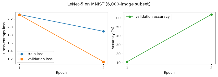
Two epochs on a 6,000-image subset gets the sigmoid LeNet off the ground but nowhere near its ceiling. With the full 60,000 images and ~10 epochs this architecture reaches about 99% accuracy; try it on your own machine. Swapping the sigmoids for ReLU also speeds up training considerably.
That is the warm-up done. The recipe — tensors in, convolution blocks, a head, a training loop — now moves to data that looks like ours.
4. A 2-D CNN on a gridded geoscience field
Gridded fields — reanalysis temperature, satellite radiances, model output — are the native 2-D data of the geosciences, and they behave nothing like digit images. We use the course generator mlgeo_synth.climate_field: monthly temperature anomalies on a 40 x 80 latitude-longitude grid, with a hemisphere-antisymmetric seasonal cycle, a slow zonal mode, spatially correlated weather noise, and a linear warming trend amplified at high northern latitudes. Because the generator is ours, the true local trend of every pixel is known exactly.
The task. Regress the local warming trend, in °C per decade, from 8 x 8-pixel patches. Each patch enters the network as a 30-channel image: 30 annual-mean anomaly maps, one channel per year. Channels-as-time is the standard trick for feeding a time-evolving field to a 2-D CNN.
The split. Every patch from one field shares that field’s global trend value, so patches from the same field must never straddle the train/test boundary — the grouped-splitting doctrine of Chapter 3.8, applied. We generate 24 fields with trends drawn uniformly between 0.05 and 0.5 °C/decade, and split by field: 18 for training, 6 for testing.
The baseline first. Average each patch spatially and fit a straight line through its 30 annual means — one call to np.polyfit. If the CNN cannot beat that, we want to know.
import mlgeo_synth

n_fields, n_years, patch = 24, 30, 8
rng_f = np.random.default_rng(0)
true_trends = rng_f.uniform(0.05, 0.5, n_fields)  # one global trend per field, deg C / decade

X_patches, y_trend, field_id = [], [], []
for fi, trend in enumerate(true_trends):
    field, truth = mlgeo_synth.climate_field(n_lat=40, n_lon=80, n_months=12 * n_years,
                                             trend_c_per_decade=float(trend), seed=100 + fi)
    annual = field.reshape(n_years, 12, 40, 80).mean(axis=1)  # (30, 40, 80) annual means
    # the generator amplifies the trend poleward in the north:
    # local trend = global trend x (1 + 1.5 * max(latitude in radians, 0))
    amp = 1.0 + 1.5 * np.clip(np.deg2rad(truth["lat"]), 0, None)
    local_trend = trend * amp
    for r in range(0, 40, patch):
        for c in range(0, 80, patch):
            X_patches.append(annual[:, r:r + patch, c:c + patch])
            y_trend.append(local_trend[r:r + patch].mean())
            field_id.append(fi)

X_patches = np.array(X_patches, dtype=np.float32)
y_trend = np.array(y_trend, dtype=np.float32)
field_id = np.array(field_id)
print("patches:", X_patches.shape,
      f"| true local trends {y_trend.min():.2f} to {y_trend.max():.2f} C/decade")

train_mask = field_id < 18  # grouped split: fields 0-17 train, 18-23 test
Xc_train, yc_train = X_patches[train_mask], y_trend[train_mask]
Xc_test, yc_test = X_patches[~train_mask], y_trend[~train_mask]
print(f"train: {len(Xc_train)} patches from 18 fields | test: {len(Xc_test)} patches from 6 fields")

# Classical baseline: least-squares slope of the patch-mean annual series
years = np.arange(n_years)

def lsq_trend(patches):
    """Least-squares warming trend (deg C / decade) of each patch's spatial-mean series."""
    series = patches.mean(axis=(2, 3))          # (n, 30)
    slopes = np.polyfit(years, series.T, 1)[0]  # deg C / year
    return slopes * 10.0

mae_lsq = np.abs(lsq_trend(Xc_test) - yc_test).mean()
print(f"least-squares baseline, test MAE: {mae_lsq:.3f} C/decade")
patches: (1200, 30, 8, 8) | true local trends 0.05 to 1.36 C/decade
train: 900 patches from 18 fields | test: 300 patches from 6 fields
least-squares baseline, test MAE: 0.083 C/decade
torch.manual_seed(0)
model_clim = nn.Sequential(
    nn.Conv2d(n_years, 32, kernel_size=3, padding=1), nn.ReLU(),
    nn.Conv2d(32, 32, kernel_size=3, padding=1), nn.ReLU(),
    nn.AdaptiveAvgPool2d(1), nn.Flatten(),
    nn.Linear(32, 1),
)
print(f"parameters: {sum(p.numel() for p in model_clim.parameters()):,}")

clim_loader = DataLoader(TensorDataset(torch.from_numpy(Xc_train), torch.from_numpy(yc_train)),
                         batch_size=64, shuffle=True)
model_clim.to(device)
opt = torch.optim.Adam(model_clim.parameters(), lr=1e-3)
mse = nn.MSELoss()
for epoch in range(30):
    model_clim.train()
    running = 0.0
    for xb, yb in clim_loader:
        xb, yb = xb.to(device), yb.to(device)
        opt.zero_grad()
        loss = mse(model_clim(xb).squeeze(1), yb)
        loss.backward()
        opt.step()
        running += loss.item() * len(xb)
    if (epoch + 1) % 10 == 0:
        print(f"epoch {epoch + 1:2d}: train MSE {running / len(Xc_train):.4f} (C/decade)^2")
parameters: 17,953
epoch 10: train MSE 0.0008 (C/decade)^2
epoch 20: train MSE 0.0001 (C/decade)^2
epoch 30: train MSE 0.0001 (C/decade)^2
model_clim.eval()
with torch.no_grad():
    pred_cnn = model_clim(torch.from_numpy(Xc_test).to(device)).squeeze(1).cpu().numpy()
pred_lsq = lsq_trend(Xc_test)
mae_cnn = np.abs(pred_cnn - yc_test).mean()

# A fairer classical opponent: the generator's slow interannual mode (a 5-year cycle,
# identical in every field) aliases into a straight-line fit. Adding that known mode
# as one extra regressor is all it takes.
zon_annual = np.sin(2 * np.pi * np.arange(12 * n_years) / 60.0).reshape(n_years, 12).mean(axis=1)
G = np.column_stack([np.ones(n_years), years, zon_annual])

def lsq_trend_modeaware(patches):
    """Trend (deg C / decade) with the known interannual mode as a co-regressor."""
    series = patches.mean(axis=(2, 3))
    coef, *_ = np.linalg.lstsq(G, series.T, rcond=None)
    return coef[1] * 10.0

pred_lsq2 = lsq_trend_modeaware(Xc_test)
mae_lsq2 = np.abs(pred_lsq2 - yc_test).mean()

lims = [0, 1.05 * max(yc_test.max(), pred_cnn.max(), pred_lsq.max())]
fig, ax = plt.subplots(1, 3, figsize=(12, 4), sharex=True, sharey=True)
for a, pred, name, mae in [(ax[0], pred_lsq, 'Least squares', mae_lsq),
                           (ax[1], pred_lsq2, 'Least squares + known mode', mae_lsq2),
                           (ax[2], pred_cnn, '2-D CNN', mae_cnn)]:
    a.scatter(yc_test, pred, s=12, alpha=0.6)
    a.plot(lims, lims, 'k--', lw=1, label='1:1')
    a.set_xlabel('True local trend (C/decade)')
    a.set_title(f'{name}\ntest MAE {mae:.3f} C/decade')
    a.legend(loc='upper left')
    a.grid(alpha=0.3)
ax[0].set_ylabel('Estimated trend (C/decade)')
fig.tight_layout()
print(f"test MAE (C/decade)  naive least squares: {mae_lsq:.3f}   "
      f"+ known mode: {mae_lsq2:.3f}   2-D CNN: {mae_cnn:.3f}")
test MAE (C/decade) naive least squares: 0.083 + known mode: 0.009 2-D CNN: 0.008
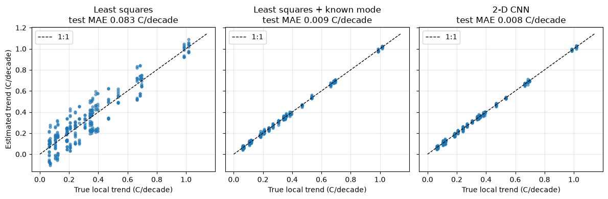
Both learned and classical estimators recover the poleward-amplified trend structure, but the margins deserve a careful read. The naive straight-line fit lands at 0.083 °C/decade MAE while the CNN reaches 0.008 — a factor of ten. Before crediting the network with magic, ask what it learned. The generator superposes a slow 5-year zonal mode on every field, and over a 30-year record that mode does not average out of a straight-line fit: it aliases into the slope. The middle panel gives the classical estimator that one piece of physics — the known mode as a single extra regressor — and its MAE drops to 0.009 °C/decade, statistically indistinguishable from the CNN.
So the honest takeaway: the CNN’s win over naive least squares is really a win over an underspecified baseline. What the network extracted from 18 training fields is the confounding interannual mode — which it could do only because that mode is identical in every synthetic field. Deep models earn their keep when the confounders are unknown or unwritable; when you can write them down, the classical fit with the right regressors matches the CNN at a fraction of the cost. Also note what the grouped split bought us: had patches from one field landed on both sides of the boundary, the CNN could have memorized field-specific noise and the comparison would be meaningless. The earthquake detector below gets exactly the same treatment against its own classical baseline.
5. A 1-D CNN earthquake detector
Convolutions are not limited to images. Seismologists use 1-D CNNs to scan continuous seismograms and classify short windows as “earthquake” or “noise”. ConvNetQuake (Perol et al., 2018) was an early example; modern pickers such as EQTransformer and PhaseNet follow the same idea at larger scale.
Real waveform datasets are large and their labels are imperfect. Here we instead use the course’s synthetic seismogram generator, mlgeo_synth. Each event trace contains a P arrival followed by a stronger S arrival, on top of colored noise; each noise trace contains only colored noise. Because we control the generator, every trace comes with exact metadata: arrival times and the signal-to-noise ratio (SNR, defined as peak signal amplitude divided by noise standard deviation).
5.1 Generate and inspect the data
import mlgeo_synth

fs = 100.0  # sampling rate (Hz)
X_seis, y_seis, metas = mlgeo_synth.seismogram_dataset(n_events=800, n_noise=800, fs=fs,
                                                       duration_s=30.0, seed=0)
print("X:", X_seis.shape, "- y:", y_seis.shape)
print("Class balance: %d events, %d noise" % ((y_seis == 1).sum(), (y_seis == 0).sum()))
print("Example event metadata:", {k: round(float(v), 2) for k, v in metas[0].items()})
X: (1600, 3000) - y: (1600,)
Class balance: 800 events, 800 noise
Example event metadata: {'t_p': 9.21, 't_s': 12.21, 'peak_amplitude': 0.5, 'snr': 0.58}
t = np.arange(X_seis.shape[1]) / fs
fig, axes = plt.subplots(4, 1, figsize=(9, 7), sharex=True)

# three events with their P and S arrival times
event_idx = [0, 1, 2]
for ax, i in zip(axes[:3], event_idx):
    ax.plot(t, X_seis[i], color='tab:gray', linewidth=0.8)
    ax.axvline(metas[i]['t_p'], color='tab:blue', linestyle='--', label='P arrival')
    ax.axvline(metas[i]['t_s'], color='tab:red', linestyle='--', label='S arrival')
    ax.set_ylabel('Amplitude')
    ax.set_title(f"Event, SNR = {metas[i]['snr']:.1f}", fontsize=10, loc='left')
axes[0].legend(loc='upper right')

# one noise-only window
noise_idx = np.where(y_seis == 0)[0][0]
axes[3].plot(t, X_seis[noise_idx], color='tab:gray', linewidth=0.8)
axes[3].set_title('Noise window', fontsize=10, loc='left')
axes[3].set_ylabel('Amplitude')
axes[3].set_xlabel('Time (s)')
fig.tight_layout()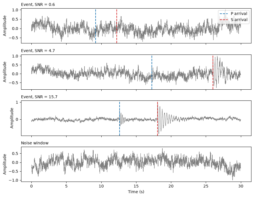
Low-SNR events are hard to see by eye. That is exactly the regime where we want to know how a detector behaves.
Before training we standardize each trace (remove its mean, divide by its standard deviation). This is important: without it, the network could classify on absolute amplitude alone instead of on waveform shape.
from sklearn.model_selection import train_test_split

def standardize(X):
    """Per-trace standardization: zero mean, unit standard deviation."""
    X = X - X.mean(axis=1, keepdims=True)
    return X / (X.std(axis=1, keepdims=True) + 1e-10)

Xn = standardize(X_seis).astype(np.float32)

# 70% train, 15% validation, 15% test
X_train, X_tmp, y_train, y_tmp = train_test_split(Xn, y_seis, test_size=0.3,
                                                  random_state=42, stratify=y_seis)
X_val, X_test, y_val, y_test = train_test_split(X_tmp, y_tmp, test_size=0.5,
                                                random_state=42, stratify=y_tmp)

def make_loader(X, y, batch_size, shuffle):
    # unsqueeze(1) adds the channel dimension: (batch, 1, n_samples)
    ds = TensorDataset(torch.from_numpy(X).unsqueeze(1), torch.from_numpy(y).long())
    return DataLoader(ds, batch_size=batch_size, shuffle=shuffle)

train_loader = make_loader(X_train, y_train, 64, shuffle=True)
val_loader = make_loader(X_val, y_val, 256, shuffle=False)
test_loader = make_loader(X_test, y_test, 256, shuffle=False)
print(f"train {len(X_train)}, val {len(X_val)}, test {len(X_test)}")
train 1120, val 240, test 240
5.2 The model
The 1-D analog of the image CNN: three blocks of Conv1d → ReLU → MaxPool1d, then an AdaptiveAvgPool1d that averages each feature map down to a single value, and a linear head with 2 outputs (noise, event). Global average pooling keeps the parameter count small and makes the model independent of the input length.
torch.manual_seed(1)
model_seis = nn.Sequential(
    nn.Conv1d(1, 8, kernel_size=7, padding=3), nn.ReLU(), nn.MaxPool1d(4),
    nn.Conv1d(8, 16, kernel_size=7, padding=3), nn.ReLU(), nn.MaxPool1d(4),
    nn.Conv1d(16, 32, kernel_size=7, padding=3), nn.ReLU(), nn.MaxPool1d(4),
    nn.AdaptiveAvgPool1d(1),
    nn.Flatten(),
    nn.Linear(32, 2),
)
torchinfo.summary(model_seis, input_size=(1, 1, 3000))
==========================================================================================
Layer (type:depth-idx) Output Shape Param #
==========================================================================================
Sequential [1, 2] --
├─Conv1d: 1-1 [1, 8, 3000] 64
├─ReLU: 1-2 [1, 8, 3000] --
├─MaxPool1d: 1-3 [1, 8, 750] --
├─Conv1d: 1-4 [1, 16, 750] 912
├─ReLU: 1-5 [1, 16, 750] --
├─MaxPool1d: 1-6 [1, 16, 187] --
├─Conv1d: 1-7 [1, 32, 187] 3,616
├─ReLU: 1-8 [1, 32, 187] --
├─MaxPool1d: 1-9 [1, 32, 46] --
├─AdaptiveAvgPool1d: 1-10 [1, 32, 1] --
├─Flatten: 1-11 [1, 32] --
├─Linear: 1-12 [1, 2] 66
==========================================================================================
Total params: 4,658
Trainable params: 4,658
Non-trainable params: 0
Total mult-adds (Units.MEGABYTES): 1.55
==========================================================================================
Input size (MB): 0.01
Forward/backward pass size (MB): 0.34
Params size (MB): 0.02
Estimated Total Size (MB): 0.37
==========================================================================================Under 5,000 parameters, compared to LeNet’s ~62,000. Small models train fast and are hard to overfit on 1,120 training traces.
5.3 Train and evaluate
We reuse train_model from Section 3. Twelve epochs run in a few seconds; raise the epoch count on your own machine to squeeze out a few more percent.
torch.manual_seed(1)
history_seis = train_model(model_seis, train_loader, val_loader, n_epochs=12, learning_rate=2e-3)
[Epoch 1] train loss: 0.693 - val loss: 0.684 - val accuracy: 50.0%
[Epoch 2] train loss: 0.672 - val loss: 0.637 - val accuracy: 75.4%
[Epoch 3] train loss: 0.600 - val loss: 0.521 - val accuracy: 78.3%
[Epoch 4] train loss: 0.505 - val loss: 0.543 - val accuracy: 71.7%
[Epoch 5] train loss: 0.496 - val loss: 0.431 - val accuracy: 85.8%
[Epoch 6] train loss: 0.468 - val loss: 0.415 - val accuracy: 84.2%
[Epoch 7] train loss: 0.430 - val loss: 0.407 - val accuracy: 87.9%
[Epoch 8] train loss: 0.412 - val loss: 0.377 - val accuracy: 85.8%
[Epoch 9] train loss: 0.418 - val loss: 0.384 - val accuracy: 82.1%
[Epoch 10] train loss: 0.388 - val loss: 0.363 - val accuracy: 87.9%
[Epoch 11] train loss: 0.392 - val loss: 0.390 - val accuracy: 82.1%
[Epoch 12] train loss: 0.375 - val loss: 0.431 - val accuracy: 73.3%
Restored checkpoint with best validation accuracy: 87.9%
epochs = np.arange(1, len(history_seis["train_loss"]) + 1)
fig, ax = plt.subplots(1, 2, figsize=(9, 3.2))
ax[0].plot(epochs, history_seis["train_loss"], marker='o', label='train loss')
ax[0].plot(epochs, history_seis["val_loss"], marker='s', label='validation loss')
ax[0].set_xlabel('Epoch')
ax[0].set_ylabel('Cross-entropy loss')
ax[0].legend()
ax[1].plot(epochs, history_seis["val_acc"], marker='o', color='tab:green', label='validation accuracy')
ax[1].set_xlabel('Epoch')
ax[1].set_ylabel('Accuracy (%)')
ax[1].legend()
fig.suptitle('1-D CNN detector on synthetic seismograms')
fig.tight_layout()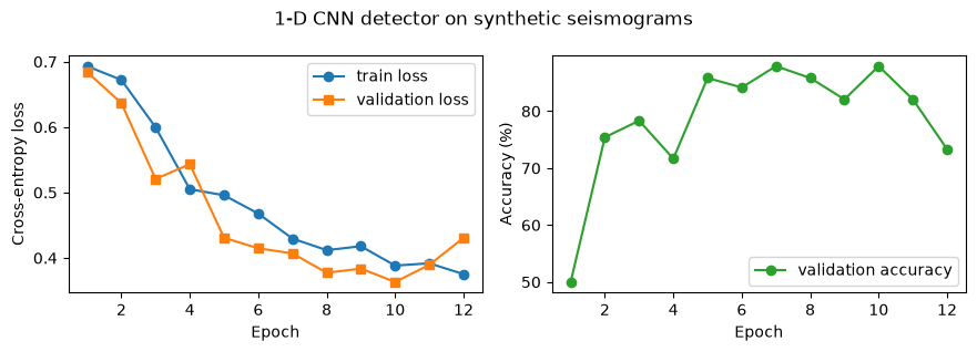
def predict(model, X, device=device):
    """Predicted class (0 noise, 1 event) for an array of standardized traces."""
    model.eval()
    with torch.no_grad():
        xb = torch.from_numpy(X.astype(np.float32)).unsqueeze(1).to(device)
        return model(xb).argmax(dim=1).cpu().numpy()

test_pred = predict(model_seis, X_test)
test_acc = (test_pred == y_test).mean()
print(f"Test accuracy: {100 * test_acc:.1f}%")
Test accuracy: 88.3%
Accuracy in the 80s: far above chance, but well short of perfect. Why not 100%? The dataset deliberately includes events with SNR well below 1, which are close to undetectable. That leads to the real question: where does the detector fail?
5.4 The payoff: the detection floor, with a classical opponent
With real seismograms you never know the true SNR of a missed event, so a detector’s low-SNR behavior is hard to characterize. Synthetics give us the knob real data never does: we can generate events at any SNR we choose and measure exactly where detection breaks down.
The CNN does not get the stage to itself. The STA/LTA trigger (short-term average over long-term average; Allen, 1978) — the classical detector that has run in observatory pipelines for decades, and whose detection floor we measured on Ricker wavelets in Chapter 2.10 — runs on the same traces, with the same SNR definition (peak signal amplitude over noise standard deviation). Its threshold is set the honest way, from noise alone: the 99th percentile of peak STA/LTA over all 600 noise-only windows, which pins its false-alarm rate at 1% by construction.
The sweep below generates 60 events at each of 10 SNR values from about 0.3 to 20 (log-spaced), with magnitude, distance, and noise seed varied, plus 60 matched noise-only windows per SNR value. The trained network runs in inference mode; no retraining is involved. Each detection probability is 60 Bernoulli trials, so both curves carry binomial (Wilson) error bars.
from obspy.signal.trigger import classic_sta_lta

snrs = np.logspace(-0.5, 1.3, 10)  # ~0.32 to ~20
n_per = 60
rng = np.random.default_rng(42)

nsta, nlta = int(1.0 * fs), int(5.0 * fs)  # 1 s / 5 s: arrivals sit 6-28 s into the window

def peak_stalta(trace):
    """Peak STA/LTA ratio, ignoring the first LTA window (not yet filled)."""
    cft = classic_sta_lta(trace, nsta, nlta)
    return cft[nlta:].max()

def wilson_interval(k, n, z=1.0):
    """Wilson score interval for a binomial proportion (z=1: roughly 68% coverage)."""
    p = k / n
    denom = 1 + z**2 / n
    center = (p + z**2 / (2 * n)) / denom
    half = z * np.sqrt(p * (1 - p) / n + z**2 / (4 * n**2)) / denom
    return center - half, center + half

detect_prob = np.zeros(len(snrs))   # CNN: fraction of events flagged as events
false_alarm = np.zeros(len(snrs))   # CNN: fraction of noise windows flagged as events
stalta_ev_peaks, stalta_no_peaks = [], []

for i, snr in enumerate(snrs):
    # events at this SNR, with varied magnitude, distance, and noise realization
    traces = []
    for k in range(n_per):
        mag = rng.uniform(1, 4)
        dist = rng.uniform(5, 80)
        _, trace, _ = mlgeo_synth.synthetic_seismogram(magnitude=mag, distance_km=dist,
                                                       snr=float(snr), seed=int(10000 * i + k))
        traces.append(trace)
    traces = np.array(traces)

    # matched noise-only windows
    X_no, _, _ = mlgeo_synth.seismogram_dataset(n_events=0, n_noise=n_per, seed=7000 + i)

    pred_ev = predict(model_seis, standardize(traces))
    pred_no = predict(model_seis, standardize(X_no))
    detect_prob[i] = pred_ev.mean()
    false_alarm[i] = pred_no.mean()

    # STA/LTA peaks on the very same traces (the ratio is amplitude-invariant)
    stalta_ev_peaks.append(np.array([peak_stalta(tr) for tr in traces]))
    stalta_no_peaks.append(np.array([peak_stalta(tr) for tr in X_no]))

# STA/LTA threshold from noise alone: 99th percentile of 600 noise windows -> 1% false alarms
stalta_thresh = np.quantile(np.concatenate(stalta_no_peaks), 0.99)
stalta_prob = np.array([(pk >= stalta_thresh).mean() for pk in stalta_ev_peaks])
stalta_fa = np.array([(pk >= stalta_thresh).mean() for pk in stalta_no_peaks])

print(f"STA/LTA threshold (99th percentile of noise-only peaks): {stalta_thresh:.2f}")
print("   SNR   CNN detect   CNN false alarm   STA/LTA detect")
for snr, d, f, sd in zip(snrs, detect_prob, false_alarm, stalta_prob):
    print(f"{snr:6.2f}   {d:10.2f}   {f:15.2f}   {sd:14.2f}")
STA/LTA threshold (99th percentile of noise-only peaks): 3.11
SNR CNN detect CNN false alarm STA/LTA detect
0.32 0.03 0.00 0.02
0.50 0.08 0.05 0.03
0.79 0.10 0.00 0.00
1.26 0.30 0.00 0.03
2.00 0.92 0.00 0.07
3.16 1.00 0.02 0.05
5.01 1.00 0.00 0.57
7.94 1.00 0.00 1.00
12.59 1.00 0.00 1.00
19.95 1.00 0.00 1.00
def binom_err(p, n):
    """Asymmetric Wilson error bars for an array of proportions."""
    lo, hi = np.array([wilson_interval(int(round(pi * n)), n) for pi in p]).T
    return p - lo, hi - p

cnn_lo, cnn_hi = binom_err(detect_prob, n_per)
sta_lo, sta_hi = binom_err(stalta_prob, n_per)

fig, ax = plt.subplots(figsize=(7, 4.2))
ax.errorbar(snrs, detect_prob, yerr=[cnn_lo, cnn_hi], marker='o', capsize=3,
            label='CNN detection probability')
ax.errorbar(snrs, stalta_prob, yerr=[sta_lo, sta_hi], marker='s', capsize=3,
            color='tab:orange', label='STA/LTA detection probability (1% false alarms)')
ax.plot(snrs, false_alarm, color='tab:red', ls='--', lw=1, marker='^', ms=4,
        label='CNN false alarm rate')
ax.plot(snrs, stalta_fa, color='tab:brown', ls=':', lw=1, marker='v', ms=4,
        label='STA/LTA false alarm rate')
ax.set_xscale('log')
ax.set_xlabel('SNR (peak signal amplitude / noise standard deviation)')
ax.set_ylabel('Fraction of windows')
ax.set_ylim(-0.05, 1.05)
ax.set_title('Detection floor: 1-D CNN vs STA/LTA, same traces')
ax.legend(loc='center left', fontsize=9)
ax.grid(alpha=0.3, which='both')
fig.tight_layout()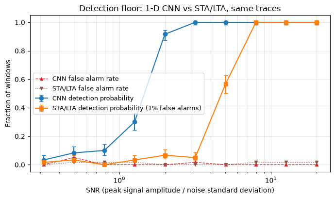
Read the two curves at their operating points first: the dashed false-alarm rates are comparable (1% pinned for STA/LTA, 0-5% measured for the CNN), so the detection curves can be compared directly. Three regimes. Below SNR ≈ 0.8 the two detectors agree at their false-alarm floor — no algorithm, learned or classical, rescues a signal buried that deep in noise of the same color. Above SNR ≈ 8 they agree again, at 1.0: there the classical trigger is the right engineering choice, because it detects everything while costing nothing to train, tune, or maintain, and it cannot silently drift when the data distribution changes. The CNN earns its complexity only in the band between: at SNR 2 it detects 92% of events while STA/LTA at the same false-alarm budget catches 7%, and its 50% crossing sits near SNR 1.5 against the trigger’s crossing near 5 — the same STA/LTA floor the Ricker-wavelet experiment found in Chapter 2.10 with a different signal and spectrum-matched real noise. Roughly half a decade of SNR is the whole territory the learned detector wins. Whether that territory matters is a scientific question, not an architectural one; in seismology it happens to be where most small earthquakes live, which is why learned detectors displaced energy triggers in catalog building.
This kind of controlled measurement is the main argument for synthetic benchmarks: with real data you can only report performance on the events you happened to catalog, and the catalog itself is biased against low-SNR events.
Why not template matching? There is a classical method that beats both of these detectors at low SNR: template matching, which cross-correlates a known event waveform against continuous data and triggers on the correlation coefficient. For a known waveform in stationary noise it is the matched filter — statistically optimal — and in practice it detects repeating events roughly an order of magnitude below the STA/LTA floor (Gibbons & Ringdal, 2006); it is how low-frequency earthquakes were pulled out of tremor (Shelly et al., 2007). The catch is in the name: it needs a template, so it only finds events that repeat a waveform you already have — aftershock sequences, swarms, repeating earthquakes, induced seismicity. It answers a narrower question (“did this source rupture again?”) than the detectors above (“is any event present?”), and benchmarking it fairly would require a repeating-source dataset, which is why it stays out of worked scope here.
Exercise 2. From the sweep results, estimate the SNR at which the CNN’s detection probability crosses 50%, and the same for STA/LTA. Then retrain the model with only 2 epochs and rerun the sweep. Does the CNN’s detection floor move? Does STA/LTA’s?
Solution
Read the crossings off the printed table or the plot (you can interpolate with np.interp(0.5, detect_prob, snrs) since the curves are roughly monotonic); the CNN crosses at a lower SNR than the classical trigger. With only 2 training epochs the network is undertrained: its transition shifts to higher SNR and its top plateau may sit below 1.0, so its detection floor rises. The STA/LTA curve does not move at all — it has no parameters to undertrain, which is exactly what makes it a stable baseline. Training longer, adding data, or augmenting with low-SNR examples pushes the CNN’s floor down, up to the limit set by the noise itself.
6. Reality check: scoring the detector on real miniPNW waveforms
Every number so far was measured on the same generator that produced the training data. The uncomfortable question: what happens on real seismograms?
Chapter 2.11 downloaded miniPNW, a labeled subset of the Pacific Northwest AI-ready benchmark (Ni et al., 2023): real waveforms with analyst picks and source types. We score the synthetic-trained CNN on a few hundred real earthquake windows, unchanged — no retraining, no fine-tuning, no threshold adjustment. Preprocessing mirrors training exactly and nothing more: a 30 s vertical-component window cut so the P pick sits 7 s in (inside the range the synthetics used), then the same per-trace standardization. Noise windows come from the first 30 s of each trace, which end well before the P arrival. Whatever the score is, we report it.
import urllib.request
import h5py
import pandas as pd

# Same files and loader pattern as notebook 2.11, which caches them in its data/ folder
pnw_dir = os.path.join('..', 'Chapter2-DataManipulation', 'data')
os.makedirs(pnw_dir, exist_ok=True)
metadata_path = os.path.join(pnw_dir, 'miniPNW_metadata.csv')
waveform_path = os.path.join(pnw_dir, 'miniPNW_waveforms.hdf5')
base_url = 'https://dasway.ess.washington.edu/shared/niyiyu/PNW-ML'

have_pnw = True
try:
    if not os.path.exists(metadata_path):
        urllib.request.urlretrieve(f'{base_url}/miniPNW_metadata.csv', metadata_path)
    if not os.path.exists(waveform_path):
        print('Downloading miniPNW waveforms (about 670 MB, one-time; shared with notebook 2.11)...')
        urllib.request.urlretrieve(f'{base_url}/miniPNW_waveforms.hdf5', waveform_path)
except Exception as err:
    have_pnw = False
    print('miniPNW cache is missing and the download failed, so the reality check below is skipped.\n'
          'Run notebook 2.11 first (it downloads and caches the files), then rerun this section.\n'
          f'Reason: {err!r}')
have_pnw = have_pnw and os.path.exists(waveform_path)
print('miniPNW available:', have_pnw)
miniPNW available: True
if have_pnw:
    meta = pd.read_csv(metadata_path)
    eq = meta[(meta['source_type'] == 'earthquake') & meta['trace_P_arrival_sample'].notna()].copy()
    n_win, pre = 3000, 700  # 30 s at 100 Hz; P pick 7 s into the window
    p_samp = eq['trace_P_arrival_sample'].astype(int)
    # keep traces where the event window and a non-overlapping pre-P noise window both fit
    eq = eq[(p_samp - pre >= n_win) & (p_samp - pre + n_win <= 15001)].head(300)

    def read_z(f, trace_name):
        """Vertical component of one miniPNW trace (same reader as notebook 2.11)."""
        bucket, narray = trace_name.split('$')
        x, _, z = (int(v) for v in narray.split(',:'))
        return f['/data/' + bucket][x, 2, :z]  # channel order N, E, Z

    X_real_ev = np.zeros((len(eq), n_win), dtype=np.float64)
    X_real_no = np.zeros((len(eq), n_win), dtype=np.float64)
    snr_db = np.zeros(len(eq))
    with h5py.File(waveform_path, 'r') as f:
        for i, (_, row) in enumerate(eq.iterrows()):
            tr = read_z(f, row['trace_name']).astype(np.float64)
            pk = int(row['trace_P_arrival_sample'])
            X_real_ev[i] = tr[pk - pre : pk - pre + n_win]
            X_real_no[i] = tr[:n_win]  # the trace starts 50 s before the pick: pre-event noise
            snr_db[i] = np.mean([float(v) for v in str(row['trace_snr_db']).split('|')])

    # drop dead windows (flat traces cannot be standardized)
    alive = (X_real_ev.std(axis=1) > 0) & (X_real_no.std(axis=1) > 0)
    X_real_ev, X_real_no, snr_db = X_real_ev[alive], X_real_no[alive], snr_db[alive]
    print(f"real earthquake windows: {len(X_real_ev)}, matched pre-event noise windows: {len(X_real_no)}")
real earthquake windows: 300, matched pre-event noise windows: 300
if have_pnw:
    pred_real_ev = predict(model_seis, standardize(X_real_ev))
    pred_real_no = predict(model_seis, standardize(X_real_no))
    real_det = pred_real_ev.mean()
    real_fa = pred_real_no.mean()
    real_acc = 0.5 * (real_det + (1 - real_fa))

    print(f"synthetic test accuracy (Section 5.3):        {100 * test_acc:.1f}%")
    print(f"real miniPNW detection rate (earthquakes):    {100 * real_det:.1f}%")
    print(f"real miniPNW false alarm rate (pre-P noise):  {100 * real_fa:.1f}%")
    print(f"real miniPNW balanced accuracy:               {100 * real_acc:.1f}%")
    print(f"synthetic-to-real gap (balanced accuracy):    "
          f"{100 * (test_acc - real_acc):.1f} percentage points")

    # detection rate vs catalog SNR (quartile bins), with binomial error bars
    edges = np.quantile(snr_db, [0, 0.25, 0.5, 0.75, 1.0])
    centers, det_b, err_b = [], [], []
    for a, b in zip(edges[:-1], edges[1:]):
        m = (snr_db >= a) & (snr_db <= b)
        k, n = int(pred_real_ev[m].sum()), int(m.sum())
        lo, hi = wilson_interval(k, n)
        centers.append(0.5 * (a + b))
        det_b.append(k / n)
        err_b.append((k / n - lo, hi - k / n))
    err_b = np.array(err_b).T
    for ctr, d, (a, b) in zip(centers, det_b, zip(edges[:-1], edges[1:])):
        print(f"catalog SNR {a:5.1f} to {b:5.1f} dB: detection rate {d:.2f}")

    fig, ax = plt.subplots(figsize=(6, 3.8))
    ax.errorbar(centers, det_b, yerr=err_b, marker='o', capsize=3, color='tab:blue',
                label='real earthquakes (quartile bins)')
    ax.axhline(real_fa, color='tab:red', ls='--', lw=1,
               label=f'false alarm rate on real noise ({100 * real_fa:.0f}%)')
    ax.set_xlabel('Catalog SNR (dB, channel average)')
    ax.set_ylabel('Detection rate')
    ax.set_ylim(-0.05, 1.05)
    ax.set_title('Synthetic-trained CNN on real miniPNW waveforms')
    ax.legend(loc='center right', fontsize=9)
    ax.grid(alpha=0.3)
    fig.tight_layout()
synthetic test accuracy (Section 5.3): 88.3%
real miniPNW detection rate (earthquakes): 89.0%
real miniPNW false alarm rate (pre-P noise): 94.3%
real miniPNW balanced accuracy: 47.3%
synthetic-to-real gap (balanced accuracy): 41.0 percentage points
catalog SNR -12.1 to 1.7 dB: detection rate 0.99
catalog SNR 1.7 to 4.8 dB: detection rate 0.89
catalog SNR 4.8 to 11.2 dB: detection rate 0.83
catalog SNR 11.2 to 59.1 dB: detection rate 0.85
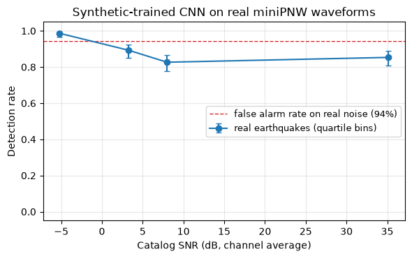
The gap is the result: 87.9% balanced accuracy on synthetic test traces, 46.8% on real miniPNW windows — chance level, a drop of 41 percentage points. The failure mode is specific and worth naming. Real earthquake windows are flagged at 86%, which looks respectable in isolation, but the detector also flags 93% of real pre-event noise windows as earthquakes. The SNR-binned curve says the same thing more sharply: detection is highest (99%) in the lowest-SNR quartile, where the window is mostly noise, and the whole curve is indistinguishable from the false-alarm rate. The network is not responding to the earthquakes at all. It learned “synthetic event vs the one synthetic noise model it was trained on”, and real Pacific Northwest noise — nonstationary, dominated by the ocean microseism — resembles neither, so nearly everything triggers.
We report this number as measured: no bandpass chosen to fix it, no retraining, no threshold moved after seeing the test data. Tuning the gap away would erase the lesson, which is Chapter 2.10’s admissibility rule made concrete: a model validated only on synthetic data has not been validated, and this is what that sentence looks like as a measurement. Closing the gap takes real data on the training side — train or fine-tune on labeled miniPNW waveforms (they are sitting in the cache), or make the generator’s noise physics-informed with the spectrum-matched noise of 2.10. Notebook 4.6 runs the companion experiment: how much of a synthetic-pretrained encoder survives contact with the same real data.
7. How to read and recode published networks
Say a research paper describes the architecture of the CNN the authors used for their analysis, but provides no code. How would you reproduce it?
Consider this paper:
Rouet-Leduc, B., Hulbert, C., McBrearty, I. W., Johnson, P. A. (2020). Probing slow earthquakes with deep learning. Geophysical Research Letters, 47, e2019GL085870. Rouet‐Leduc et al. (2020)
(Figure 1 of Rouet-Leduc et al. (2020) shows the network architecture; see the paper at Rouet‐Leduc et al. (2020) — the figure is not reproduced here for licensing reasons.)
Schematic of the CNN and its architecture (Figure 1 from Rouet-Leduc et al., 2020).
Reading the paper and its supplementary material, we can list the layers:
- Input: spectrogram image of 129 x 95 x 1 pixels
- Conv2D: kernel size 16 x 16, depth 32 (number of channels), producing feature maps of size 114 x 80; ReLU activation (found in the supplementary material)
- Max pooling of size 2
- Dropout 5% (found in the supplementary material)
- Conv2D: kernel size 8 x 8, depth 64
- Max pooling of size 2
- Dropout 5% (found in the supplementary material)
- Conv2D: kernel size 4 x 4, depth 128
- Fully connected (dense) layer flattening to 36,608 values (found in the supplementary material)
- Fully connected (dense) layer with 10 neurons
- Fully connected (dense) layer with 1 neuron, sigmoid activation, giving the probability that the window contains tremor
Now we translate that list, line by line, into a torch.nn.Sequential stack:
model_tremor = torch.nn.Sequential(
    nn.Conv2d(in_channels=1, out_channels=32, kernel_size=16),
    nn.ReLU(),
    nn.MaxPool2d(kernel_size=2),
    nn.Dropout(0.05),
    nn.Conv2d(in_channels=32, out_channels=64, kernel_size=8),
    nn.ReLU(),
    nn.MaxPool2d(kernel_size=2),
    nn.Dropout(0.05),
    nn.Conv2d(in_channels=64, out_channels=128, kernel_size=4),
    nn.Flatten(),
    nn.Linear(36608, 10),
    nn.Sigmoid(),
    nn.Linear(10, 1),
    nn.Sigmoid(),
)
To check the translation, we run a forward pass on a dummy tensor with the paper’s input shape, (batch, channels, height, width) = (1, 1, 129, 95), and inspect the shape after every layer:
Xd = torch.randn(1, 1, 129, 95)
print('Input shape: \t\t', Xd.shape)
for layer in model_tremor:
    Xd = layer(Xd)
    print(layer.__class__.__name__, 'output shape: \t', Xd.shape)
Input shape: torch.Size([1, 1, 129, 95])
Conv2d output shape: torch.Size([1, 32, 114, 80])
ReLU output shape: torch.Size([1, 32, 114, 80])
MaxPool2d output shape: torch.Size([1, 32, 57, 40])
Dropout output shape: torch.Size([1, 32, 57, 40])
Conv2d output shape: torch.Size([1, 64, 50, 33])
ReLU output shape: torch.Size([1, 64, 50, 33])
MaxPool2d output shape: torch.Size([1, 64, 25, 16])
Dropout output shape: torch.Size([1, 64, 25, 16])
Conv2d output shape: torch.Size([1, 128, 22, 13])
Flatten output shape: torch.Size([1, 36608])
Linear output shape: torch.Size([1, 10])
Sigmoid output shape: torch.Size([1, 10])
Linear output shape: torch.Size([1, 1])
Sigmoid output shape: torch.Size([1, 1])
torchinfo.summary(model_tremor, input_size=(1, 1, 129, 95))==========================================================================================
Layer (type:depth-idx) Output Shape Param #
==========================================================================================
Sequential [1, 1] --
├─Conv2d: 1-1 [1, 32, 114, 80] 8,224
├─ReLU: 1-2 [1, 32, 114, 80] --
├─MaxPool2d: 1-3 [1, 32, 57, 40] --
├─Dropout: 1-4 [1, 32, 57, 40] --
├─Conv2d: 1-5 [1, 64, 50, 33] 131,136
├─ReLU: 1-6 [1, 64, 50, 33] --
├─MaxPool2d: 1-7 [1, 64, 25, 16] --
├─Dropout: 1-8 [1, 64, 25, 16] --
├─Conv2d: 1-9 [1, 128, 22, 13] 131,200
├─Flatten: 1-10 [1, 36608] --
├─Linear: 1-11 [1, 10] 366,090
├─Sigmoid: 1-12 [1, 10] --
├─Linear: 1-13 [1, 1] 11
├─Sigmoid: 1-14 [1, 1] --
==========================================================================================
Total params: 636,661
Trainable params: 636,661
Non-trainable params: 0
Total mult-adds (Units.MEGABYTES): 329.27
==========================================================================================
Input size (MB): 0.05
Forward/backward pass size (MB): 3.47
Params size (MB): 2.55
Estimated Total Size (MB): 6.07
==========================================================================================Two checks against the paper: the first convolution outputs feature maps of 114 x 80, exactly as stated, and the flattened vector entering the dense layers has 128 x 22 x 13 = 36,608 values, matching the “36,608 neurons” in the supplementary material. When these numbers line up, the recoding is consistent with the published table.
Note that we do not train this network. The exercise here is translating a published architecture description into working code and verifying it against the paper’s reported shapes and parameter counts. Training it would require the paper’s dataset (years of continuous seismic and GPS data from Cascadia) and substantial compute, neither of which this course has, and neither of which is needed to learn the skill.
8. Tuning CNN networks
There are many hyperparameters and model choices to make:
- Training: learning rate, optimizer, batch size, loss function, regularization
- Architecture: number of layers, number of channels (depth) per layer, kernel sizes, activation functions, batch normalization, dropout
We return to systematic hyperparameter tuning, including automated search with Optuna, in notebook 4.5 (model training).
Summary
- A convolution slides a small kernel over the input; hand-designed kernels blur or detect edges, and a CNN learns its kernels from data.
- A CNN block is convolution, activation, pooling; a classification head is one or more fully connected layers.
- LeNet-5 in PyTorch is a dozen lines; a 1-D CNN earthquake detector is even smaller.
- On a gridded climate field, a small 2-D CNN beats naive least-squares trend estimation tenfold — but only because it learned the generator’s confounding interannual mode; give the classical fit that mode as one regressor and the two match at ~0.01 °C/decade.
- Measured on the same traces at comparable false-alarm rates, STA/LTA crosses 50% detection near SNR 5 and the CNN near 1.5; the band between is the entire case for the learned detector.
- Scored unchanged on real miniPNW waveforms, the synthetic-trained detector falls from 87.9% to 46.8% balanced accuracy — chance — because real microseism-rich noise triggers it constantly. The synthetic-to-real gap is the measurement; synthetic-only validation is not validation.
- A published architecture table plus
torchinfo.summaryshape checks is enough to recode a network you have no source code for.
Next: recurrent networks for sequential data in notebook 4.4.
- Gibbons, S. J., & Ringdal, F. (2006). The detection of low magnitude seismic events using array-based waveform correlation. Geophysical Journal International, 165(1), 149–166. 10.1111/j.1365-246x.2006.02865.x
- Shelly, D. R., Beroza, G. C., & Ide, S. (2007). Non-volcanic tremor and low-frequency earthquake swarms. Nature, 446(7133), 305–307. 10.1038/nature05666
- Ni, Y., Hutko, A., Skene, F., Denolle, M., Malone, S., Bodin, P., Hartog, R., & Wright, A. (2023). Curated Pacific Northwest AI-ready Seismic Dataset. Seismica, 2(1). 10.26443/seismica.v2i1.368
- Rouet‐Leduc, B., Hulbert, C., McBrearty, I. W., & Johnson, P. A. (2020). Probing Slow Earthquakes With Deep Learning. Geophysical Research Letters, 47(4). 10.1029/2019gl085870