Homework Deep Learning (75 points) - Machine Learning in the Geosciences

In this homework, we will build an earthquake detector: a classifier that decides whether a 30-second window of 100 Hz vertical-component ground motion contains an earthquake or only noise. The windows come from the course package mlgeo_synth with a fixed seed, so every event has a known magnitude, distance, and signal-to-noise ratio; the instructor holds a hidden-seed variant used to spot-check submitted results.

This is the same detection task as the 1-D CNN in lesson 4.3, on a fresh dataset and with a different model family. An MLP has no translation invariance: it cannot learn that an earthquake at second 8 and an earthquake at second 14 are the same thing. We therefore feed it the log amplitude spectrum of each window, which discards arrival time and keeps the frequency content that separates events (band-limited wavelet energy) from noise (a power-law spectrum). Chapter 2.6 built this transform; here it earns its keep.

We will practice the skills of lessons 4.1, 4.2, and 4.5: build and train an MLP in PyTorch, run a controlled architecture experiment, diagnose broken training runs from their curves, evaluate honestly against a baseline, and quantify uncertainty with a small deep ensemble.

Importing Libraries¶

import numpy as np
import matplotlib.pyplot as plt
import torch
import torch.nn as nn
from sklearn.model_selection import train_test_split
from sklearn.preprocessing import StandardScaler
from sklearn.linear_model import LogisticRegression
%matplotlib inline

1. Build and Train an MLP Detector (20 points)¶

We follow the following steps:

inspect the data (2 points)
leakage-aware split and scaling (4 points)
complete the model skeleton (4 points)
write the training loop (8 points)
learning curves (2 points)

import mlgeo_synth

fs = 100.0  # sampling rate (Hz)
X_wave, y, metas = mlgeo_synth.seismogram_dataset(
    n_events=600, n_noise=600, fs=fs, duration_s=30.0, seed=2026)
print(X_wave.shape, y.shape)

(1200, 3000) (1200,)

Each row of X_wave is one 30 s window (3000 samples); y is 1 for event windows and 0 for noise windows. For event windows, metas records the true P and S arrival times and the signal-to-noise ratio.

The cell below computes the model input: the log amplitude spectrum of each window, restricted to the 0.2–30 Hz band where both the wavelet energy and the noise live. This is the AI-ready representation the MLP will see.

freqs = np.fft.rfftfreq(X_wave.shape[1], d=1/fs)
band = (freqs >= 0.2) & (freqs <= 30.0)
X_spec = np.log10(np.abs(np.fft.rfft(X_wave, axis=1))[:, band] + 1e-10).astype(np.float32)
f_band = freqs[band]
print(X_spec.shape)

(1200, 895)

1.1 Inspect the data¶

Task: report the class counts, then plot one event window and one noise window — the waveform on the left, its log amplitude spectrum on the right (2 points). Label the axes with units (time in s, frequency in Hz). Use metas to mark the P and S arrival times on the event waveform.

# TODO: class counts; one event and one noise window, waveform + spectrum

1.2 Leakage-aware split and scaling¶

Task: split into train (60%), validation (20%), and test (20%) sets, stratified on the label, then standardize the spectra (4 points).

First split off the 20% test set (random_state=42, stratify=y), then split the remainder 75/25 into train and validation (random_state=42, stratified again).
Fit a StandardScaler on the training set only and apply it to all three sets. Convert the results to float32.
Name the arrays X_train, X_val, X_test and the labels y_train, y_val, y_test.

The validation set steers training decisions (architecture, stopping); the test set is touched once, in section 4. You will explain in section 4.2 what fitting the scaler on the full dataset would have leaked.

# TODO: train/val/test split, scaler fit on train only

1.3 The model skeleton¶

Task: complete the skeleton below (4 points). Two hidden layers, both of size width, a ReLU after each, and a final linear layer to n_classes outputs with no activation — nn.CrossEntropyLoss expects raw logits.

class DetectorMLP(nn.Module):
    """MLP detector: log amplitude spectrum in, 2 class logits out."""

    def __init__(self, n_in, width=32, n_classes=2):
        super().__init__()
        # TODO: define the layers

    def forward(self, x):
        # TODO: return the logits
        raise NotImplementedError

1.4 The training loop¶

Task: write a training function from scratch and train a width=32 model for 25 epochs (8 points). This is the five-step recipe of lesson 4.1 — dataset, model, loss, optimizer, loop — and you must be able to produce it unaided.

Requirements for train_detector:

minibatches of 64, reshuffled every epoch (a fresh random permutation of the training indices is enough — no DataLoader required);
nn.CrossEntropyLoss and torch.optim.Adam with lr=1e-3;
per epoch, record the mean training loss, the validation loss, and the validation accuracy in a history dictionary — compute the validation quantities under torch.no_grad() with the model in eval() mode, and put it back in train() mode afterwards;
seed everything (torch.manual_seed for the model init before construction, numpy rng for the shuffling) so a rerun reproduces your numbers.

# TODO: write train_detector(model, X_train, y_train, X_val, y_val,
#                              n_epochs=25, lr=1e-3, batch_size=64, seed=0)
#       returning history = {"train_loss": [...], "val_loss": [...], "val_acc": [...]}
#       then train a width=32 DetectorMLP with seed 0

1.5 Learning curves¶

Task: plot the training and validation loss on one panel and the validation accuracy on another (2 points). State in one sentence whether the model is overfitting, underfitting, or neither, and point to the evidence in the curves.

# TODO: learning curves

2. Architecture Experiment: Width (15 points)¶

One controlled experiment: hold everything fixed and vary the width of the hidden layers. Because a single training run is a random draw (initialization and batch order), every configuration is trained with three seeds, and the seed spread is part of the result — lesson 4.5 calls a difference smaller than the seed spread what it is: noise.

sweep (8 points)
error-bar plot (4 points)
pick and justify (3 points)

2.1 The sweep¶

Task: train a DetectorMLP for each width in [8, 32, 128] and each seed in [0, 1, 2] — nine runs — and record the final validation accuracy of each (8 points). Reuse train_detector unchanged: 25 epochs, lr=1e-3, batch size 64. The nine runs take under a minute on a laptop.

# TODO: 3 widths x 3 seeds, record final validation accuracy

2.2 Error bars¶

Task: plot validation accuracy against width (log-scaled x-axis), showing for each width the mean across seeds and error bars spanning the min–max seed spread (4 points).

# TODO: mean with min-max error bars across seeds

2.3 Pick and justify¶

Task: choose a width and defend the choice in two or three sentences (3 points). Your justification must compare the accuracy differences between widths against the seed spread, and account for parameter count: a gain that costs 16x the parameters had better be larger than the error bars.

3. Diagnose Two Broken Training Runs (10 points)¶

The cell below trains two rigged configurations on this dataset and plots, for each, the per-step training loss and the per-epoch validation accuracy. It also prints the fraction of validation windows each final model calls an event. Both runs are broken in a different way — the same pathologies lesson 4.5 taught you to read.

For each run, write down in the answer cell: the pathology (2 points), the evidence in the curves that identifies it (2 points), and the first fix you would try (1 point). Diagnose from the curves before reading the configuration code — that is the skill being graded.

def make_broken_runs():
    """Two rigged training runs. Diagnose from the curves before reading this code."""
    Xb_trainval, _, yb_trainval, _ = train_test_split(
        X_spec, y, test_size=0.2, random_state=7, stratify=y)
    Xb_train, Xb_val, yb_train, yb_val = train_test_split(
        Xb_trainval, yb_trainval, test_size=0.25, random_state=7, stratify=yb_trainval)
    scaler_b = StandardScaler().fit(Xb_train)
    Xb_train = scaler_b.transform(Xb_train).astype(np.float32)
    Xb_val = scaler_b.transform(Xb_val).astype(np.float32)

    configs = {
        "Run A": dict(lr=5.0, ordered=False, n_epochs=12),
        "Run B": dict(lr=0.5, ordered=True, n_epochs=12),
    }

    Xt, yt = torch.from_numpy(Xb_train), torch.from_numpy(yb_train)
    Xv, yv = torch.from_numpy(Xb_val), torch.from_numpy(yb_val)
    results = {}
    for name, cfg in configs.items():
        torch.manual_seed(0)
        model = nn.Sequential(
            nn.Linear(Xb_train.shape[1], 32), nn.ReLU(),
            nn.Linear(32, 32), nn.ReLU(), nn.Linear(32, 2))
        optimizer = torch.optim.SGD(model.parameters(), lr=cfg["lr"])
        loss_fn = nn.CrossEntropyLoss()
        rng = np.random.default_rng(0)
        step_loss, val_acc = [], []
        for epoch in range(cfg["n_epochs"]):
            if cfg["ordered"]:
                order = np.argsort(yb_train, kind="stable")  # noise first, events last
            else:
                order = rng.permutation(len(yb_train))
            for i in range(0, len(yb_train), 64):
                idx = order[i:i + 64]
                optimizer.zero_grad()
                loss = loss_fn(model(Xt[idx]), yt[idx])
                loss.backward()
                optimizer.step()
                step_loss.append(loss.item())
            model.eval()
            with torch.no_grad():
                pred_val = model(Xv).argmax(dim=1)
                val_acc.append((pred_val == yv).float().mean().item())
            model.train()
        results[name] = dict(step_loss=np.array(step_loss), val_acc=val_acc,
                             frac_event=pred_val.float().mean().item())
    return results


broken = make_broken_runs()

fig, axes = plt.subplots(2, 2, figsize=(10, 6))
for row, (name, res) in enumerate(broken.items()):
    ax = axes[row, 0]
    ax.semilogy(res["step_loss"])
    ax.set_xlabel("training step")
    ax.set_ylabel("training loss")
    ax.set_title(f"{name}: per-step training loss")
    ax.grid(alpha=0.3)
    ax = axes[row, 1]
    ax.plot(np.arange(1, len(res["val_acc"]) + 1), res["val_acc"], marker="o")
    ax.axhline(0.5, color="gray", ls="--", label="chance")
    ax.set_ylim(0.3, 1.0)
    ax.set_xlabel("epoch")
    ax.set_ylabel("validation accuracy")
    ax.set_title(f"{name}: validation accuracy")
    ax.legend()
    ax.grid(alpha=0.3)
    print(f"{name}: final model calls {res['frac_event']:.0%} of validation windows an event")
plt.tight_layout()

Run A: final model calls 3% of validation windows an event
Run B: final model calls 100% of validation windows an event

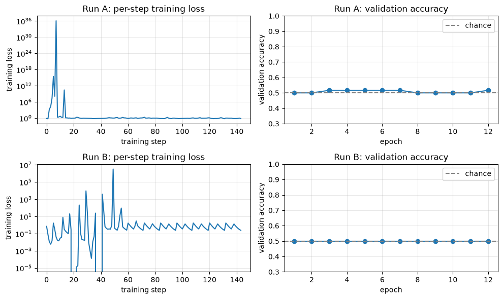
Run A

Pathology:
Evidence:
Fix:

Run B

Pathology:
Evidence:
Fix:

4. Honest Evaluation (15 points)¶

A detector score means nothing on its own. We establish what a trivial model and a linear model achieve on the same split, audit the pipeline for leakage, and report every metric with uncertainty — the design of lesson 4.5 and the leaderboard rules of 3.5 and 4.10.

baselines first (4 points)
leakage audit (3 points)
metrics with uncertainty (6 points)
verdict (2 points)

4.1 Baselines first¶

Task: compute two baselines on the test set (4 points): the majority-class baseline, and a LogisticRegression(max_iter=5000) trained on the same standardized spectra (X_train). Report both test accuracies.

# TODO: majority-class baseline and logistic-regression baseline on the test set

4.2 Leakage audit¶

Task: answer in three sentences (3 points). (1) Why must the StandardScaler be fit on the training set only — what exactly leaks if it is fit on the full dataset before splitting? (2) Why is the per-window spectrum transform (the X_spec cell) safe to apply before splitting? (3) Name one decision you made in this notebook that used the validation set, and confirm the test set played no part in it.

4.3 Metrics with uncertainty¶

A test set of 240 windows is a sample, not the truth; the helper below bootstraps it to put a confidence interval on an accuracy.

Task: report the test accuracy with a 95% bootstrap confidence interval for your trained MLP from section 1 and for the logistic-regression baseline (6 points).

def bootstrap_ci(y_true, y_pred, n_boot=2000, seed=0):
    """95% bootstrap confidence interval for accuracy."""
    rng = np.random.default_rng(seed)
    n = len(y_true)
    accs = np.empty(n_boot)
    for b in range(n_boot):
        idx = rng.integers(0, n, n)
        accs[b] = np.mean(y_true[idx] == y_pred[idx])
    return np.percentile(accs, [2.5, 97.5])

# TODO: test accuracy with 95% CI, MLP and logistic baseline

4.4 Verdict¶

Task: state whether the MLP beats the logistic baseline, using the confidence intervals, and explain the result in one or two sentences (2 points). If the intervals overlap, say so plainly — lesson 4.5’s rule applies: if your deep model cannot beat the linear baseline, the problem is the data or the features, not a missing layer. What about this representation makes a linear model so competitive, and which model from Chapter 4 would you reach for to do better on the raw waveforms?

5. Uncertainty from a Small Deep Ensemble (12 points)¶

Retraining the same architecture with different seeds gives a deep ensemble (lesson 4.5, Pillar 2): the members agree where the data speak clearly and disagree where they do not.

train 3 members (4 points)
spread versus error (5 points)
calibration statement (3 points)

5.1 Train three members¶

Task: train three width=32 models with seeds 100, 101, 102 — same data, same hyperparameters as section 1 — and collect each member’s predicted probability of “event” on the test set (4 points). Stack them into an array member_probs of shape (3, n_test) (softmax the logits and keep column 1).

# TODO: three members, member_probs of shape (3, n_test)

5.2 Spread versus error¶

Task: report the accuracy of the ensemble-mean prediction, then call plot_spread_vs_error(member_probs, y_test) and describe the pattern in one sentence (5 points). The helper bins the test windows into terciles of ensemble spread (the standard deviation of the three predicted probabilities) and plots the accuracy in each bin.

def plot_spread_vs_error(member_probs, y_true):
    """Accuracy within terciles of ensemble spread."""
    P = np.asarray(member_probs)
    mean_p, std_p = P.mean(axis=0), P.std(axis=0)
    correct = (mean_p > 0.5).astype(int) == np.asarray(y_true)
    edges = np.quantile(std_p, [0, 1/3, 2/3, 1.0])
    edges[-1] += 1e-9
    labels = ["low spread", "medium spread", "high spread"]
    accs = []
    for lo, hi in zip(edges[:-1], edges[1:]):
        in_bin = (std_p >= lo) & (std_p < hi)
        accs.append(correct[in_bin].mean())
    fig, ax = plt.subplots(figsize=(5.5, 3.5))
    ax.bar(labels, accs, edgecolor="black")
    ax.axhline(correct.mean(), color="black", ls="--",
               label=f"overall accuracy {correct.mean():.2f}")
    ax.set_ylabel("accuracy in bin")
    ax.set_ylim(0.4, 1.0)
    ax.set_title("Ensemble spread vs error")
    ax.legend()
    ax.grid(axis="y", alpha=0.3)
    return accs

# TODO: ensemble-mean accuracy, then plot_spread_vs_error(member_probs, y_test)

5.3 Calibration statement¶

Task: compare the ensemble’s mean confidence against its accuracy and write one calibration sentence (3 points). Compute the confidence of each test prediction (the larger of mean_p and 1 - mean_p), average it over the test set, and set it next to the ensemble accuracy from 5.2. Your sentence must name the direction and rough size of the miscalibration — for example: “the ensemble claims X% confidence but is right Y% of the time, so it is overconfident by about Z points”.

# TODO: mean confidence vs accuracy

6. AI-Use Disclosure (3 points)¶

Every submission in this course carries a disclosure (1.8, 6.4). Fill in the table: one row per tool, stating the task it did and what you verified. The third column is the one that gets graded — “verified nothing” is at least honest and costs less than a verification claim that collapses under one question. If you used no assistant, write one row saying so. Remember that the training loop of 1.4 and the diagnoses of section 3 were 🔒 By hand: they must not appear as assistant tasks here, and you may be asked to defend them orally.

Task: complete the disclosure table (3 points).

Tool	Task	What I verified

Instructor grading notes

Reference numbers below come from the reference solution (seed 2026 data, 25 epochs, Adam lr=1e-3, batch 64). Implementation choices (shuffling rng, tensor dtype) shift accuracies by 1–2 points; grade the reasoning, and use the hidden-seed variant to spot-check any result that looks copied rather than run.

1. MLP (20 pts). 1.1 (2): counts 600/600; event waveform with P and S marked, spectra show band-limited bump vs power-law noise. 1.2 (4): split 60/20/20 stratified; full credit requires the scaler fit on X_train only — fitting on the full data loses 2. 1.3 (4): two hidden layers of width with ReLU, linear head, no softmax in forward (softmax in forward: −1). 1.4 (8): 🔒 by hand. Look for: fresh permutation each epoch (2), correct zero_grad/backward/step order (2), validation in eval() + no_grad and back to train() (2), history recorded per epoch and seeding (2). A DataLoader loop is acceptable. 1.5 (2): curves plus one supported sentence — expected: mild gap, “neither” or “slight overfitting” both defensible.

2. Width experiment (15 pts). 2.1 (8): nine runs, final val accuracy each; reference means ≈ 0.81 (w=8), 0.83 (w=32), 0.85 (w=128) with seed spread ≈ ±0.01–0.02. 2.2 (4): mean with min–max bars, log x-axis. 2.3 (3): any width is acceptable if the argument compares gaps against spread and mentions parameter cost; “128 because biggest number” without the spread comparison earns 1.

3. Broken runs (10 pts, 🔒 by hand). Run A — learning rate too high (SGD, lr=5.0). Evidence: per-step loss explodes to ~1e36 in the first epochs and keeps spiking on the log axis; validation accuracy sits at chance for all 12 epochs; the final model calls ~3% of validation windows an event. Fix: cut the learning rate by 10–100x (or switch to Adam at 1e-3). Run B — batches not shuffled and sorted by class (ordered=True: all noise batches, then all event batches, identical order every epoch). Evidence: validation accuracy pinned at exactly 0.50 for all 12 epochs while the per-step training loss looks healthy (~0.4–0.7) and repeats an identical sawtooth every epoch; the printed line shows the final model calls 100% of validation windows an event — it see-saws to whatever class it saw last. Fix: shuffle the training data every epoch. Per run: pathology 2, evidence 2, fix 1. Accept “class-ordered data / no shuffling” phrasings; “overfitting” for Run B earns 0 for the pathology point.

4. Honest evaluation (15 pts). 4.1 (4): majority baseline 0.50; logistic regression ≈ 0.85 test accuracy. 4.2 (3): one point per sentence — (1) full-data scaler leaks test-set means/variances into training inputs; (2) the spectrum is computed per window from that window alone, so no cross-window statistics flow; (3) width choice used validation only. 4.3 (6): MLP ≈ 0.83 [0.78, 0.88], logistic ≈ 0.85 [0.81, 0.90] — CI half-width ≈ ±0.045. 4.4 (2): expected verdict — the intervals overlap; the MLP does not beat the linear baseline. The log-spectrum representation nearly linearizes the problem (log spectral amplitude vs class is close to linearly separable); the model to reach for on raw waveforms is the 1-D CNN of 4.3. Penalize claims of MLP superiority built on point estimates the CIs contradict.

5. Ensemble (12 pts). 5.1 (4): seeds 100/101/102, member test accuracies ≈ 0.82–0.85. 5.2 (5): ensemble-mean accuracy ≈ 0.83; tercile accuracies ≈ 0.96 / 0.85 / 0.69 — monotone decline, i.e. spread ranks errors. 5.3 (3): mean confidence ≈ 0.87 vs accuracy ≈ 0.83 → overconfident by ≈ 4 points; the sentence must state direction and magnitude, not just “reasonably calibrated”.

6. Disclosure (3 pts). Graded per 6.4: specific tasks and concrete verification earn 3; empty or generic (“checked it looks right”) earns 1; a disclosure that lists 🔒 sections as assistant work triggers the oral defense.