An autoencoder is a neural network trained to reproduce its own input. That sounds pointless until you add a constraint: the network must squeeze the data through a narrow bottleneck before reconstructing it. To succeed, the network has to learn a compact representation that keeps the structure of the data and discards the rest.
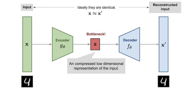
The architecture has three parts and is usually symmetric:
- the encoder compresses the input into a small set of features (linear layers, convolutional layers, ...),
- the bottleneck (or latent space) is the smallest layer, the low-dimensional representation of the data,
- the decoder takes the latent features and reconstructs the original data.
Because the training target is the input itself, no labels are needed. This is the simplest form of self-supervised learning, and it is why autoencoders matter: after training, the encoder is a feature extractor learned from unlabeled data. Autoencoders are used for compression, denoising, feature extraction, and anomaly detection.
In this notebook we build three autoencoders on spectrograms of synthetic seismograms: a dense autoencoder, a convolutional autoencoder, and a denoising autoencoder that maps noisy spectrograms to clean ones. We finish with a masked-autoencoder demo — run on two domains, seismic spectrograms and gridded climate fields — and transfer experiments, including one onto real miniPNW waveforms, that show why the trained encoder is the part worth keeping, and how far its features carry.
A good overview of autoencoder variants: Lilian Weng’s blog post.
🖥️ Lecture slides — Session 26 (Wed Dec 2, enrichment context)
import os
import numpy as np
import matplotlib.pyplot as plt
import scipy.signal
import torch
import torch.nn as nn
from torch.utils.data import DataLoader, TensorDataset
from torchinfo import summary

from mlgeo_synth import seismogram_dataset, synthetic_seismogram

device = torch.device("cuda" if torch.cuda.is_available()
                      else "mps" if torch.backends.mps.is_available()
                      else "cpu")
print("device:", device)

torch.manual_seed(0)
rng = np.random.default_rng(0)
device: cpu
1. A spectrogram dataset from synthetic seismograms
We generate 600 event seismograms and 600 noise seismograms with mlgeo_synth (30 s at 100 Hz, so 3000 samples each). Instead of feeding raw waveforms to the network, we work with log-spectrograms: time-frequency images computed with the short-time Fourier transform. Spectrograms turn a 1D signal into a 2D image, which lets us reuse everything we know about convolutional networks. This is also what research denoisers like DeepDenoiser do (more on that in Section 4).
The spectrogram parameters are chosen so that every image has the same size: nperseg=128 gives 65 frequency bins (we drop the DC bin to get 64) and noverlap=83 gives exactly 64 time frames for a 3000-sample trace. We take log10 of the power with a small floor to avoid log(0), then normalize with a single global min and max so that all images live in [0, 1] on the same scale. A shared scale matters later, when the input and the target of the denoiser must be comparable.
# Generate the waveform dataset
X_wave, y_lab, metas = seismogram_dataset(n_events=600, n_noise=600, fs=100.0,
                                          duration_s=30.0, seed=0)
print("waveforms:", X_wave.shape, "| events:", int(y_lab.sum()), "| noise:", int((1 - y_lab).sum()))

FS = 100.0
NPERSEG, NOVERLAP = 128, 83
EPS = 1e-12

def log_spectrogram(trace):
    """Return a 64x64 log-power spectrogram of a 3000-sample trace."""
    f, t, Sxx = scipy.signal.spectrogram(trace, fs=FS, nperseg=NPERSEG, noverlap=NOVERLAP)
    return np.log10(Sxx[1:, :] + EPS), f[1:], t   # drop the DC bin -> 64 x 64

# Compute all spectrograms
S0, freqs, times = log_spectrogram(X_wave[0])
X_spec = np.zeros((len(X_wave),) + S0.shape, dtype=np.float32)
for i, tr in enumerate(X_wave):
    X_spec[i] = log_spectrogram(tr)[0]

# Global normalization to [0, 1] -- store the constants for reuse
S_MIN, S_MAX = X_spec.min(), X_spec.max()
def normalize(spec):
    return np.clip((spec - S_MIN) / (S_MAX - S_MIN), 0.0, 1.0).astype(np.float32)

X_img = normalize(X_spec)
print("images:", X_img.shape, "| range:", X_img.min(), "-", X_img.max())
waveforms: (1200, 3000) | events: 600 | noise: 600
images: (1200, 64, 64) | range: 0.0 - 1.0
# Show a few spectrograms with their labels
fig, axs = plt.subplots(2, 4, figsize=(10, 4.5), sharex=True, sharey=True)
idx_ev = np.where(y_lab == 1)[0][:4]
idx_no = np.where(y_lab == 0)[0][:4]
for k in range(4):
    axs[0, k].pcolormesh(times, freqs, X_img[idx_ev[k]], cmap="viridis", vmin=0, vmax=1)
    axs[0, k].set_title(f"event (snr={metas[idx_ev[k]]['snr']:.1f})", fontsize=9)
    axs[1, k].pcolormesh(times, freqs, X_img[idx_no[k]], cmap="viridis", vmin=0, vmax=1)
    axs[1, k].set_title("noise", fontsize=9)
for ax in axs[1, :]:
    ax.set_xlabel("time (s)")
for ax in axs[:, 0]:
    ax.set_ylabel("frequency (Hz)")
plt.tight_layout()
plt.show()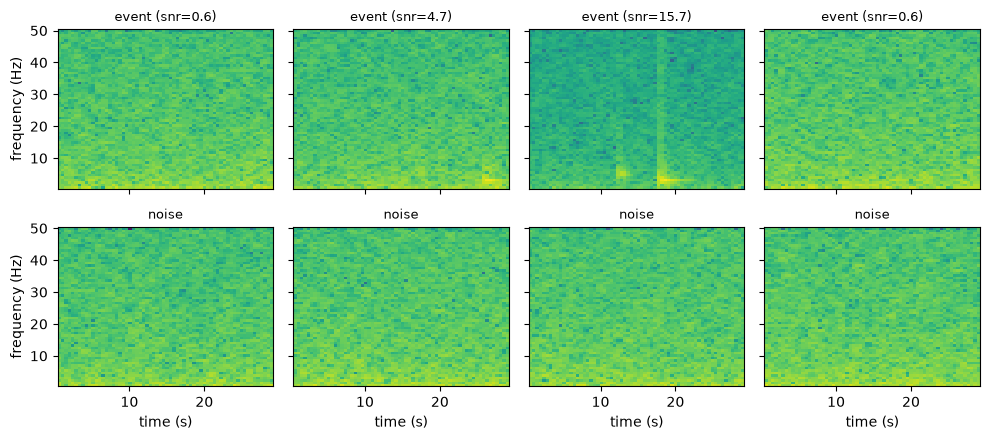
The events show the classic signature: an impulsive onset, energy concentrated at the source corner frequency, and a coda that decays with time. Noise fills the whole image more evenly. Note that low-SNR events are hard to spot by eye, which is the point of building a denoiser later.
1.1 Train/validation split and data loaders
We split 80/20 and wrap the images in PyTorch DataLoaders. Each loader yields (input, target) pairs. For a plain autoencoder the target is the input itself.
n = len(X_img)
perm = rng.permutation(n)
n_train = int(0.8 * n)
itrain, ival = perm[:n_train], perm[n_train:]

# Tensors with a channel dimension: (N, 1, 64, 64)
T_train = torch.from_numpy(X_img[itrain]).unsqueeze(1)
T_val = torch.from_numpy(X_img[ival]).unsqueeze(1)
y_train = torch.from_numpy(y_lab[itrain]).long()
y_val = torch.from_numpy(y_lab[ival]).long()

train_loader = DataLoader(TensorDataset(T_train, T_train), batch_size=64, shuffle=True)
val_loader = DataLoader(TensorDataset(T_val, T_val), batch_size=64, shuffle=False)

# validation examples used for display: the highest-SNR events, easiest to see
snr_val = np.array([metas[j]["snr"] if y_lab[j] == 1 else 0.0 for j in ival])
disp = torch.from_numpy(np.argsort(snr_val)[::-1][:6].copy())
print("train:", T_train.shape, "| val:", T_val.shape)
train: torch.Size([960, 1, 64, 64]) | val: torch.Size([240, 1, 64, 64])
2. Dense autoencoder
The first autoencoder uses only fully connected layers. The 64x64 image is flattened to a 4096-dimensional vector, compressed to a latent vector of 32 numbers (a 128x compression), then expanded back. The final Sigmoid keeps the output in [0, 1], matching the normalized images.
LATENT = 32

class DenseEncoder(nn.Module):
    def __init__(self, latent=LATENT):
        super().__init__()
        self.net = nn.Sequential(
            nn.Flatten(),
            nn.Linear(64 * 64, 256), nn.SELU(),
            nn.Linear(256, latent), nn.SELU(),   # bottleneck
        )
    def forward(self, x):
        return self.net(x)

class DenseDecoder(nn.Module):
    def __init__(self, latent=LATENT):
        super().__init__()
        self.net = nn.Sequential(
            nn.Linear(latent, 256), nn.SELU(),
            nn.Linear(256, 64 * 64), nn.Sigmoid(),
        )
    def forward(self, x):
        return self.net(x).view(-1, 1, 64, 64)

class AutoEncoder(nn.Module):
    """Generic wrapper: any encoder followed by any decoder."""
    def __init__(self, encoder, decoder):
        super().__init__()
        self.encoder = encoder
        self.decoder = decoder
    def forward(self, x):
        return self.decoder(self.encoder(x))

dense_ae = AutoEncoder(DenseEncoder(), DenseDecoder()).to(device)
summary(dense_ae, input_size=(64, 1, 64, 64), device=device)
==========================================================================================
Layer (type:depth-idx) Output Shape Param #
==========================================================================================
AutoEncoder [64, 1, 64, 64] --
├─DenseEncoder: 1-1 [64, 32] --
│ └─Sequential: 2-1 [64, 32] --
│ │ └─Flatten: 3-1 [64, 4096] --
│ │ └─Linear: 3-2 [64, 256] 1,048,832
│ │ └─SELU: 3-3 [64, 256] --
│ │ └─Linear: 3-4 [64, 32] 8,224
│ │ └─SELU: 3-5 [64, 32] --
├─DenseDecoder: 1-2 [64, 1, 64, 64] --
│ └─Sequential: 2-2 [64, 4096] --
│ │ └─Linear: 3-6 [64, 256] 8,448
│ │ └─SELU: 3-7 [64, 256] --
│ │ └─Linear: 3-8 [64, 4096] 1,052,672
│ │ └─Sigmoid: 3-9 [64, 4096] --
==========================================================================================
Total params: 2,118,176
Trainable params: 2,118,176
Non-trainable params: 0
Total mult-adds (Units.MEGABYTES): 135.56
==========================================================================================
Input size (MB): 1.05
Forward/backward pass size (MB): 2.38
Params size (MB): 8.47
Estimated Total Size (MB): 11.90
==========================================================================================2.1 Training function
One function trains every model in this notebook. It reads (input, target) pairs from the loader, so the same code handles plain reconstruction (target = input), denoising (target = clean image), and masking (target = full image). The loss is the mean squared error between the reconstruction and the target.
def train_ae(model, train_loader, val_loader=None, n_epochs=8, lr=1e-3, print_every=1):
    criterion = nn.MSELoss()
    optimizer = torch.optim.Adam(model.parameters(), lr=lr)
    loss_train = np.zeros(n_epochs)
    loss_val = np.zeros(n_epochs)
    for epoch in range(n_epochs):
        model.train()
        running = 0.0
        for xb, tb in train_loader:
            xb, tb = xb.to(device), tb.to(device)
            optimizer.zero_grad()
            loss = criterion(model(xb), tb)
            loss.backward()
            optimizer.step()
            running += loss.item()
        loss_train[epoch] = running / len(train_loader)
        if val_loader is not None:
            model.eval()
            running = 0.0
            with torch.no_grad():
                for xb, tb in val_loader:
                    xb, tb = xb.to(device), tb.to(device)
                    running += criterion(model(xb), tb).item()
            loss_val[epoch] = running / len(val_loader)
            if (epoch + 1) % print_every == 0:
                print(f"[epoch {epoch+1:2d}] train loss: {loss_train[epoch]:.4f}"
                      f" - val loss: {loss_val[epoch]:.4f}")
        elif (epoch + 1) % print_every == 0:
            print(f"[epoch {epoch+1:2d}] train loss: {loss_train[epoch]:.4f}")
    return loss_train, loss_val
loss_d, loss_dv = train_ae(dense_ae, train_loader, val_loader, n_epochs=8, lr=1e-3)
plt.figure(figsize=(5, 3))
plt.plot(np.arange(1, len(loss_d) + 1), loss_d, label="training loss")
plt.plot(np.arange(1, len(loss_dv) + 1), loss_dv, label="validation loss")
plt.xlabel("epoch"); plt.ylabel("MSE loss"); plt.legend(); plt.title("Dense autoencoder")
plt.tight_layout(); plt.show()[epoch 1] train loss: 0.0293 - val loss: 0.0054
[epoch 2] train loss: 0.0049 - val loss: 0.0040
[epoch  3] train loss: 0.0039 - val loss: 0.0036
[epoch  4] train loss: 0.0035 - val loss: 0.0034
[epoch  5] train loss: 0.0032 - val loss: 0.0033
[epoch  6] train loss: 0.0032 - val loss: 0.0030
[epoch  7] train loss: 0.0033 - val loss: 0.0035
[epoch  8] train loss: 0.0043 - val loss: 0.0038
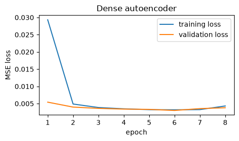
A note on compute: 8 epochs on 960 small images is enough to see the behavior. On your own machine, raise the epochs or the dataset size for sharper reconstructions.
2.2 Input vs reconstruction
def show_reconstruction(model, inputs, targets=None, n_images=5, row_titles=None):
    """Top row: inputs. Middle (optional): targets. Bottom: model reconstructions."""
    model.eval()
    with torch.no_grad():
        recon = model(inputs[:n_images].to(device)).cpu().numpy().squeeze(1)
    rows = [inputs[:n_images].numpy().squeeze(1), recon]
    if targets is not None:
        rows.append(targets[:n_images].numpy().squeeze(1))
    if row_titles is None:
        row_titles = ["input", "reconstruction", "target"][: len(rows)]
    fig, axs = plt.subplots(len(rows), n_images, figsize=(2 * n_images, 2 * len(rows)))
    for r in range(len(rows)):
        for c in range(n_images):
            axs[r, c].imshow(rows[r][c], origin="lower", cmap="viridis", vmin=0, vmax=1)
            axs[r, c].set_xticks([]); axs[r, c].set_yticks([])
        axs[r, 0].set_ylabel(row_titles[r])
    plt.tight_layout(); plt.show()

show_reconstruction(dense_ae, T_val[disp], n_images=6)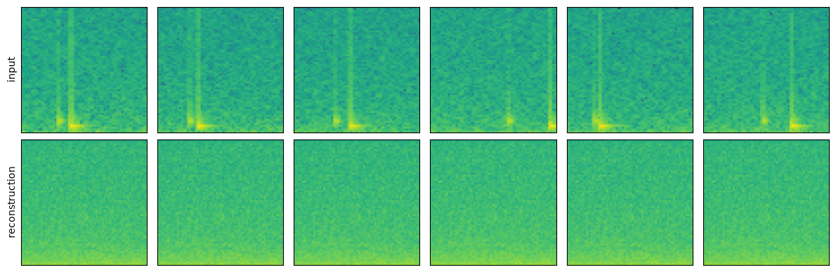
The dense autoencoder reproduces the smooth part of each image, the background level and the bright low-frequency band, but the sharp arrivals are gone. Flattening the image throws away the 2D neighborhood structure, and 32 latent numbers cannot store where a thin vertical stripe sits.
3. Convolutional autoencoder
Convolutional layers respect the 2D structure of the spectrogram. The encoder halves the image three times with strided convolutions (64 -> 32 -> 16 -> 8), and the decoder mirrors it with ConvTranspose2d layers. We add BatchNorm2d after each convolution, standard practice that speeds up and stabilizes training.
The bottleneck is now a 64x8x8 feature map. Count the numbers: 4096, the same as the input. The compression here is spatial, not in raw count: each of the 8x8 positions must summarize an 8x8 patch of the image in 64 features, so the network still cannot copy pixels through. Different bottleneck shapes impose different constraints, and we return to that below.
class ConvEncoder(nn.Module):
    def __init__(self):
        super().__init__()
        self.net = nn.Sequential(
            nn.Conv2d(1, 16, 3, stride=2, padding=1),   # -> 16 x 32 x 32
            nn.BatchNorm2d(16), nn.ReLU(),
            nn.Conv2d(16, 32, 3, stride=2, padding=1),  # -> 32 x 16 x 16
            nn.BatchNorm2d(32), nn.ReLU(),
            nn.Conv2d(32, 64, 3, stride=2, padding=1),  # -> 64 x 8 x 8
            nn.BatchNorm2d(64), nn.ReLU(),
        )
    def forward(self, x):
        return self.net(x)

class ConvDecoder(nn.Module):
    def __init__(self):
        super().__init__()
        self.net = nn.Sequential(
            nn.ConvTranspose2d(64, 32, 3, stride=2, padding=1, output_padding=1),
            nn.BatchNorm2d(32), nn.ReLU(),
            nn.ConvTranspose2d(32, 16, 3, stride=2, padding=1, output_padding=1),
            nn.BatchNorm2d(16), nn.ReLU(),
            nn.ConvTranspose2d(16, 1, 3, stride=2, padding=1, output_padding=1),
            nn.Sigmoid(),
        )
    def forward(self, x):
        return self.net(x)

conv_ae = AutoEncoder(ConvEncoder(), ConvDecoder()).to(device)
summary(conv_ae, input_size=(64, 1, 64, 64), device=device)
==========================================================================================
Layer (type:depth-idx) Output Shape Param #
==========================================================================================
AutoEncoder [64, 1, 64, 64] --
├─ConvEncoder: 1-1 [64, 64, 8, 8] --
│ └─Sequential: 2-1 [64, 64, 8, 8] --
│ │ └─Conv2d: 3-1 [64, 16, 32, 32] 160
│ │ └─BatchNorm2d: 3-2 [64, 16, 32, 32] 32
│ │ └─ReLU: 3-3 [64, 16, 32, 32] --
│ │ └─Conv2d: 3-4 [64, 32, 16, 16] 4,640
│ │ └─BatchNorm2d: 3-5 [64, 32, 16, 16] 64
│ │ └─ReLU: 3-6 [64, 32, 16, 16] --
│ │ └─Conv2d: 3-7 [64, 64, 8, 8] 18,496
│ │ └─BatchNorm2d: 3-8 [64, 64, 8, 8] 128
│ │ └─ReLU: 3-9 [64, 64, 8, 8] --
├─ConvDecoder: 1-2 [64, 1, 64, 64] --
│ └─Sequential: 2-2 [64, 1, 64, 64] --
│ │ └─ConvTranspose2d: 3-10 [64, 32, 16, 16] 18,464
│ │ └─BatchNorm2d: 3-11 [64, 32, 16, 16] 64
│ │ └─ReLU: 3-12 [64, 32, 16, 16] --
│ │ └─ConvTranspose2d: 3-13 [64, 16, 32, 32] 4,624
│ │ └─BatchNorm2d: 3-14 [64, 16, 32, 32] 32
│ │ └─ReLU: 3-15 [64, 16, 32, 32] --
│ │ └─ConvTranspose2d: 3-16 [64, 1, 64, 64] 145
│ │ └─Sigmoid: 3-17 [64, 1, 64, 64] --
==========================================================================================
Total params: 46,849
Trainable params: 46,849
Non-trainable params: 0
Total mult-adds (Units.MEGABYTES): 805.85
==========================================================================================
Input size (MB): 1.05
Forward/backward pass size (MB): 56.62
Params size (MB): 0.19
Estimated Total Size (MB): 57.86
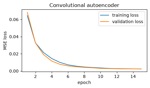
==========================================================================================loss_c, loss_cv = train_ae(conv_ae, train_loader, val_loader, n_epochs=15, lr=1e-3)
plt.figure(figsize=(5, 3))
plt.plot(np.arange(1, len(loss_c) + 1), loss_c, label="training loss")
plt.plot(np.arange(1, len(loss_cv) + 1), loss_cv, label="validation loss")
plt.xlabel("epoch"); plt.ylabel("MSE loss"); plt.legend(); plt.title("Convolutional autoencoder")
plt.tight_layout(); plt.show()[epoch 1] train loss: 0.0644 - val loss: 0.0683
[epoch 2] train loss: 0.0327 - val loss: 0.0327
[epoch 3] train loss: 0.0214 - val loss: 0.0190
[epoch 4] train loss: 0.0145 - val loss: 0.0115
[epoch 5] train loss: 0.0100 - val loss: 0.0078
[epoch 6] train loss: 0.0071 - val loss: 0.0059
[epoch 7] train loss: 0.0056 - val loss: 0.0049
[epoch 8] train loss: 0.0046 - val loss: 0.0042
[epoch 9] train loss: 0.0040 - val loss: 0.0037
[epoch 10] train loss: 0.0035 - val loss: 0.0030
[epoch 11] train loss: 0.0030 - val loss: 0.0027
[epoch 12] train loss: 0.0027 - val loss: 0.0026
[epoch 13] train loss: 0.0025 - val loss: 0.0025
[epoch 14] train loss: 0.0024 - val loss: 0.0024
[epoch 15] train loss: 0.0024 - val loss: 0.0024
show_reconstruction(conv_ae, T_val[disp], n_images=6)
print(f"validation MSE  dense: {loss_dv[-1]:.4f}   conv: {loss_cv[-1]:.4f}")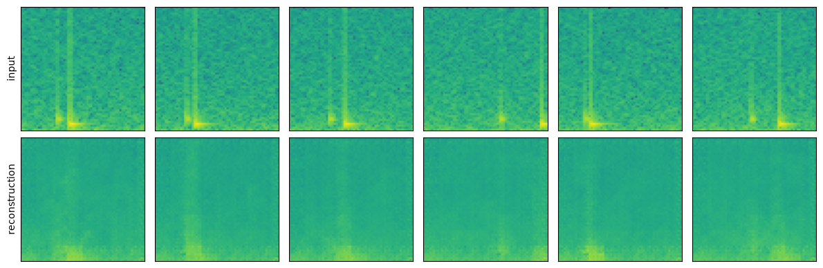
validation MSE dense: 0.0038 conv: 0.0024
The convolutional autoencoder reaches a lower validation loss than the dense one, and the reconstructions now keep a trace of the arrivals: a faint vertical stripe at the S wave and the bright patch at the onset. Still blurry, and that is inherent to bottleneck architectures: fine detail is discarded by design.
The bottleneck is a dial, not a fixed choice. The dense model squeezed to 32 numbers, a brutal compression, and lost the arrivals. The convolutional model keeps 4096 numbers arranged as a coarse spatial map, a much gentler constraint, which explains the sharper output. Shrink the bottleneck and reconstructions get blurrier but the representation gets more abstract; widen it and reconstruction improves until, at the extreme, the network can copy the input and learns nothing useful. The right latent size depends on what you want the representation for, an idea we return to in Section 6. As a home exercise, add a fourth stride-2 convolution (bottleneck 128x4x4) or project the feature map down to a 32-number vector, retrain, and watch the reconstruction quality change.
4. Denoising autoencoder: the seismology payoff
So far the network reproduces its input. A small change makes it do something genuinely useful: give it a noisy spectrogram as input and the clean spectrogram of the same event as the target. The network can no longer learn the identity; it must learn what earthquake signals look like and what noise looks like, and keep only the former.
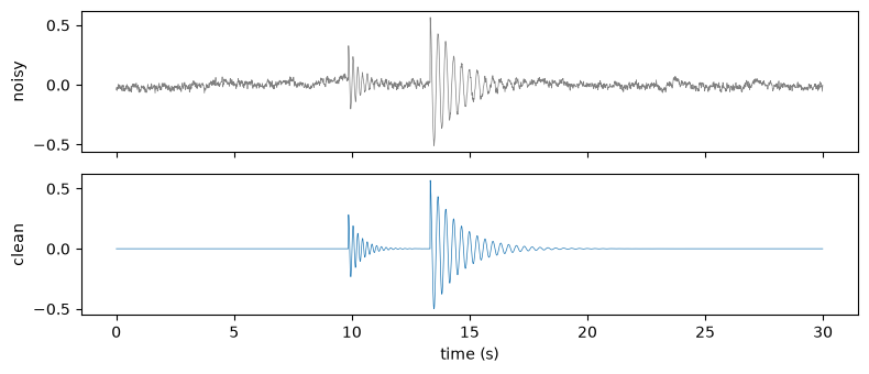
To train it we need matched clean/noisy pairs, which is exactly what a synthetic generator is for. synthetic_seismogram called twice with the same source parameters and the same seed produces the identical underlying event; only the noise amplitude changes with snr. We use snr=1e6 (noise a million times smaller than the signal, effectively clean) for the target and a random snr between 5 and 30 for the input: noisy, but with the event still present in the data. The cell below verifies the pairing: the residual between the two traces has the amplitude expected from the SNR and is uncorrelated with the signal.
n_pairs = 400
noisy_w = np.zeros((n_pairs, 3000))
clean_w = np.zeros((n_pairs, 3000))
prng = np.random.default_rng(42)
for i in range(n_pairs):
    mag = prng.uniform(1.5, 3.5)
    dist = prng.uniform(5, 60)
    snr_low = 10 ** prng.uniform(np.log10(5.0), np.log10(30.0))   # noisy input
    kw = dict(duration_s=30.0, fs=100.0, magnitude=mag, distance_km=dist, seed=1000 + i)
    _, clean_w[i], mc = synthetic_seismogram(snr=1e6, **kw)
    t, noisy_w[i], mn = synthetic_seismogram(snr=snr_low, **kw)

# Verify: same signal, different noise
resid = noisy_w[0] - clean_w[0]
print(f"identical source? peak amplitudes: {mc['peak_amplitude']:.4f} vs {mn['peak_amplitude']:.4f}")
print(f"residual std: {resid.std():.4f} (expected noise std: {mn['peak_amplitude']/mn['snr']:.4f})")
print(f"correlation of residual with clean signal: {np.corrcoef(resid, clean_w[0])[0, 1]:+.3f}")

fig, axs = plt.subplots(2, 1, figsize=(8, 3.5), sharex=True)
axs[0].plot(t, noisy_w[0], lw=0.5, color="gray"); axs[0].set_ylabel("noisy")
axs[1].plot(t, clean_w[0], lw=0.5, color="C0"); axs[1].set_ylabel("clean")
axs[1].set_xlabel("time (s)")
plt.tight_layout(); plt.show()
identical source? peak amplitudes: 0.4918 vs 0.4918
residual std: 0.0244 (expected noise std: 0.0264)
correlation of residual with clean signal: +0.004
# Spectrograms of both, normalized with the SAME global constants as before
S_noisy = np.stack([normalize(log_spectrogram(w)[0]) for w in noisy_w])
S_clean = np.stack([normalize(log_spectrogram(w)[0]) for w in clean_w])

n_tr = int(0.8 * n_pairs)
Tn_train = torch.from_numpy(S_noisy[:n_tr]).unsqueeze(1)
Tc_train = torch.from_numpy(S_clean[:n_tr]).unsqueeze(1)
Tn_val = torch.from_numpy(S_noisy[n_tr:]).unsqueeze(1)
Tc_val = torch.from_numpy(S_clean[n_tr:]).unsqueeze(1)

den_train = DataLoader(TensorDataset(Tn_train, Tc_train), batch_size=64, shuffle=True)
den_val = DataLoader(TensorDataset(Tn_val, Tc_val), batch_size=64, shuffle=False)
print("denoiser training pairs:", len(Tn_train), "| validation pairs:", len(Tn_val))
denoiser training pairs: 320 | validation pairs: 80
The architecture is unchanged: a fresh instance of the Section 3 convolutional autoencoder. Only the data changed. The task is harder than plain reconstruction, because input and target now look very different, and there is an easy shortcut: output the average dark background everywhere. That shortcut is a strong local minimum (without batch normalization the network gets stuck in it), so we train longer. The model is tiny and each epoch takes a fraction of a second.
denoiser = AutoEncoder(ConvEncoder(), ConvDecoder()).to(device)
loss_n, loss_nv = train_ae(denoiser, den_train, den_val, n_epochs=80, lr=1e-3,
                           print_every=10)
[epoch 10] train loss: 0.0933 - val loss: 0.0892
[epoch 20] train loss: 0.0355 - val loss: 0.0349
[epoch 30] train loss: 0.0208 - val loss: 0.0205
[epoch 40] train loss: 0.0151 - val loss: 0.0157
[epoch 50] train loss: 0.0122 - val loss: 0.0129
[epoch 60] train loss: 0.0102 - val loss: 0.0117
[epoch 70] train loss: 0.0090 - val loss: 0.0109
[epoch 80] train loss: 0.0079 - val loss: 0.0103
# Noisy input / denoised output / clean target triplets
show_reconstruction(denoiser, Tn_val, targets=Tc_val, n_images=5,
                    row_titles=["noisy input", "denoised output", "clean target"])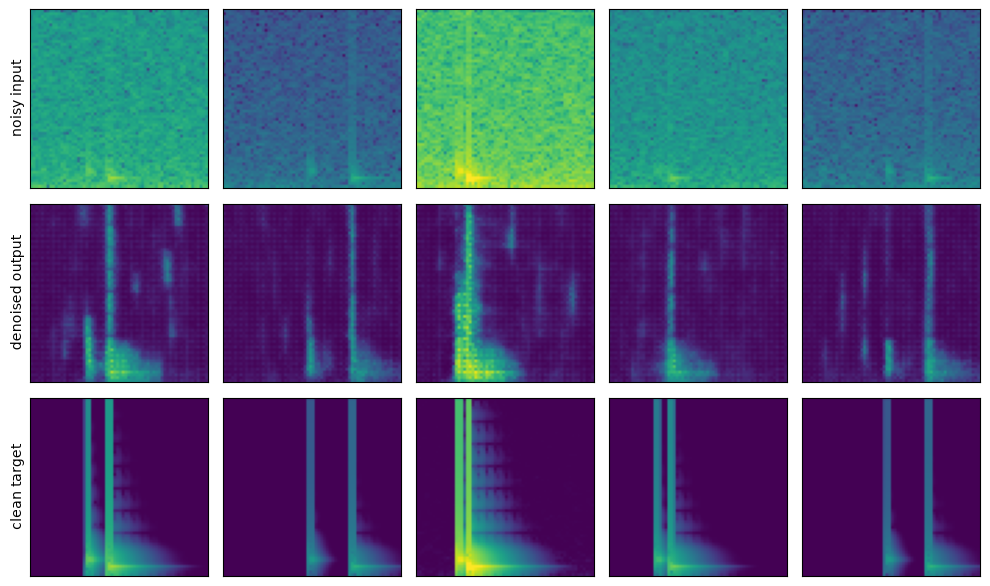
The denoiser suppresses the broadband noise floor and recovers the event energy: the S arrival, the coda, the low-frequency concentration. The output is not perfect; arrivals are smeared and low-SNR examples lose detail. But remember what this network is: six convolutional layers trained for 80 epochs on 320 image pairs.
This miniature has direct research-scale counterparts. DeepDenoiser (Zhu et al., 2019) works on the short-time Fourier transform of seismograms, exactly our input representation, and predicts time-frequency masks that separate signal from noise; it is used in production earthquake-monitoring pipelines. WaveDecompNet (Yin et al., 2022) takes the idea further with a two-branch decoder that decomposes a recording into an earthquake component and a noise component, keeping both, because the “noise” (the ambient wavefield) is itself scientifically useful. Both are encoder-decoder networks at heart; they differ from our toy in depth, in training-set size, and in the skip connections discussed in Section 7.
5. Masked autoencoder: a ten-line change
Denoising is one way to corrupt the input; masking is another. Zero out random square patches of the image and ask the network to reconstruct the full image. To fill in a missing patch, the network cannot copy pixels; it must understand context, e.g. that an event’s coda continues smoothly in time and that noise has a consistent spectral shape. The change from Section 3 is about ten lines: a masking function and a new pair of loaders.
def mask_patches(imgs, patch=8, n_patches=12, seed=0):
    """Zero out n_patches random patch x patch squares in each image."""
    g = np.random.default_rng(seed)
    masked = imgs.clone()
    N, _, H, W = imgs.shape
    for i in range(N):
        for _ in range(n_patches):
            r, c = g.integers(0, H - patch), g.integers(0, W - patch)
            masked[i, 0, r:r + patch, c:c + patch] = 0.0
    return masked

M_train = mask_patches(T_train, seed=1)
M_val = mask_patches(T_val, seed=2)
mask_train = DataLoader(TensorDataset(M_train, T_train), batch_size=64, shuffle=True)
mask_val = DataLoader(TensorDataset(M_val, T_val), batch_size=64, shuffle=False)

masked_ae = AutoEncoder(ConvEncoder(), ConvDecoder()).to(device)
loss_m, loss_mv = train_ae(masked_ae, mask_train, mask_val, n_epochs=8, lr=1e-3)
[epoch 1] train loss: 0.0614 - val loss: 0.0478
[epoch 2] train loss: 0.0298 - val loss: 0.0262
[epoch 3] train loss: 0.0167 - val loss: 0.0131
[epoch 4] train loss: 0.0097 - val loss: 0.0071
[epoch 5] train loss: 0.0062 - val loss: 0.0045
[epoch 6] train loss: 0.0044 - val loss: 0.0035
[epoch 7] train loss: 0.0035 - val loss: 0.0031
[epoch 8] train loss: 0.0031 - val loss: 0.0029
show_reconstruction(masked_ae, M_val[disp], targets=T_val[disp], n_images=5,
                    row_titles=["masked input", "reconstruction", "original"])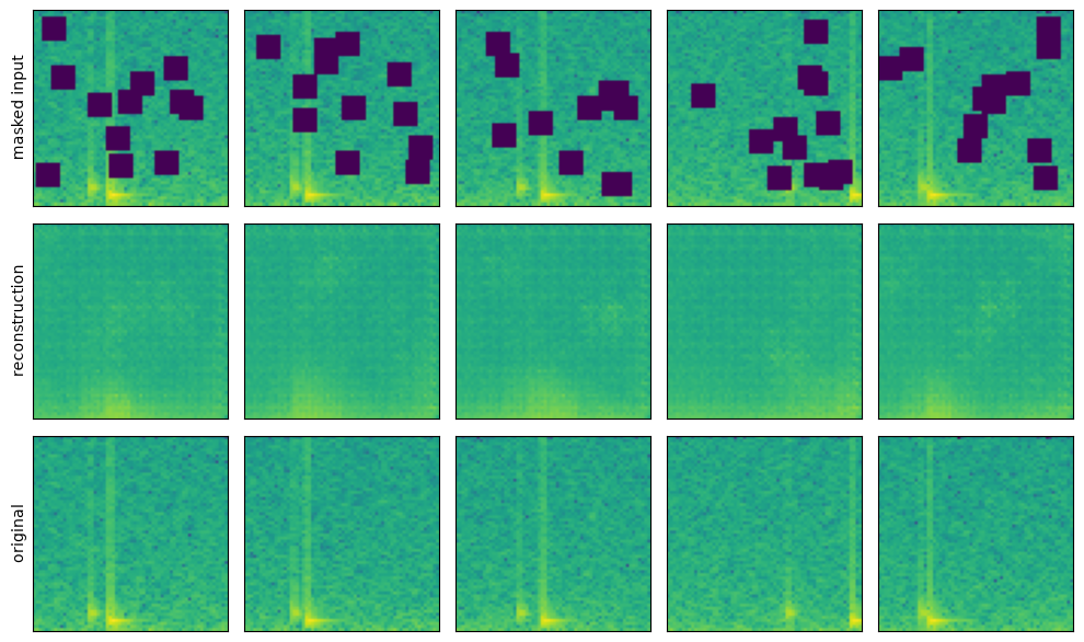
With 12 random 8x8 patches hidden, at most 18.75% of each 64x64 image (less where patches overlap), the network fills the holes with plausible time-frequency content inferred from the surroundings.
This objective, corrupt the input, predict what was removed, is the core of modern self-supervised pretraining. Masked language modeling (hide words, predict them) is how BERT-style language models are pretrained, and masked autoencoders for images (He et al., 2022) showed that hiding 75% of image patches and reconstructing them produces features that transfer well to classification and detection. No human ever labeled anything: the data supervises itself, so pretraining can consume arbitrarily large unlabeled archives.
That last point is why this matters in the geosciences. Seismic networks record continuously and accumulate petabytes of unlabeled waveforms, while analyst-labeled catalogs cover a sliver of it. A model pretrained by masking or denoising on the raw archive learns what seismic signals look like before it ever sees a label. Foundation-model efforts in seismology and remote sensing follow exactly this recipe: self-supervised pretraining on the archive, then a small supervised fine-tune for each downstream task.
5.1 The same ten lines on a second domain: climate fields
Nothing in the masking objective is seismological. To prove it, the identical architecture and the identical ten lines run on a second domain: the gridded climate-anomaly fields of Chapter 4.3. We generate two fields with mlgeo_synth.climate_field (40 x 80 latitude-longitude grid, 30 years of monthly anomalies) and treat each month’s map as one image: 720 images, normalized to [0, 1] with global constants, exactly as we treated the spectrograms. The convolutional autoencoder is fully convolutional, so the 40 x 80 maps pass through with no code change — the bottleneck is simply 64 x 5 x 10 instead of 64 x 8 x 8.
from mlgeo_synth import climate_field

C_maps = np.concatenate([
    climate_field(n_lat=40, n_lon=80, n_months=360, trend_c_per_decade=0.3, seed=sd)[0]
    for sd in (0, 1)]).astype(np.float32)          # (720, 40, 80) monthly anomaly maps
C_imgs = ((C_maps - C_maps.min()) / (C_maps.max() - C_maps.min())).astype(np.float32)

perm_c = np.random.default_rng(7).permutation(len(C_imgs))
n_ct = int(0.8 * len(C_imgs))
Ct_train = torch.from_numpy(C_imgs[perm_c[:n_ct]]).unsqueeze(1)
Ct_val = torch.from_numpy(C_imgs[perm_c[n_ct:]]).unsqueeze(1)

Cm_train, Cm_val = mask_patches(Ct_train, seed=3), mask_patches(Ct_val, seed=4)
cmask_train = DataLoader(TensorDataset(Cm_train, Ct_train), batch_size=64, shuffle=True)
cmask_val = DataLoader(TensorDataset(Cm_val, Ct_val), batch_size=64, shuffle=False)

masked_ae_clim = AutoEncoder(ConvEncoder(), ConvDecoder()).to(device)
loss_mc, loss_mcv = train_ae(masked_ae_clim, cmask_train, cmask_val, n_epochs=8, lr=1e-3)
[epoch 1] train loss: 0.0517 - val loss: 0.0481
[epoch 2] train loss: 0.0297 - val loss: 0.0468
[epoch 3] train loss: 0.0199 - val loss: 0.0456
[epoch 4] train loss: 0.0119 - val loss: 0.0318
[epoch 5] train loss: 0.0068 - val loss: 0.0098
[epoch 6] train loss: 0.0040 - val loss: 0.0045
[epoch 7] train loss: 0.0027 - val loss: 0.0023
[epoch 8] train loss: 0.0020 - val loss: 0.0021
show_reconstruction(masked_ae_clim, Cm_val[:5], targets=Ct_val[:5], n_images=5,
                    row_titles=["masked input", "reconstruction", "original"])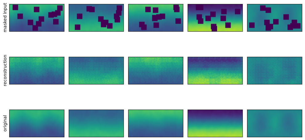
The network fills the masked squares with smooth, latitude-consistent anomaly structure and ends near a validation MSE of 0.002 on this domain: the seasonal bands and the zonal pattern give it strong context to infer from. One architecture, one objective, two Earth-science domains — that portability, not any single reconstruction, is the argument for self-supervised pretraining on gridded archives, and it is exactly the recipe behind remote-sensing and weather foundation models.
6. The encoder is what gets reused
After training, the decoder is usually thrown away. The valuable artifact is the encoder: a feature extractor learned without labels. Here is the test. The conv-autoencoder encoder from Section 3 was trained on reconstruction only; it never saw an event/noise label. We first look at its latent space, then use it for classification with very few labels.
# PCA of the frozen encoder's latent space, colored by (held-out) labels
from sklearn.decomposition import PCA

conv_ae.eval()
with torch.no_grad():
    Z_val = conv_ae.encoder(T_val.to(device)).flatten(1).cpu().numpy()
Z2 = PCA(n_components=2).fit_transform(Z_val)

plt.figure(figsize=(5, 4))
for lab, name, col in [(0, "noise", "C0"), (1, "event", "C1")]:
    m = y_val.numpy() == lab
    plt.scatter(Z2[m, 0], Z2[m, 1], s=8, c=col, label=name, alpha=0.6)
plt.xlabel("PC 1"); plt.ylabel("PC 2"); plt.legend()
plt.title("Latent space of the conv encoder (PCA)")
plt.tight_layout(); plt.show()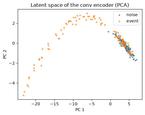
The two classes already separate, at least partly, even though no label was used in training. Now the experiment: suppose an analyst labeled only 10% of the training set (96 spectrograms). We compare two classifiers with the identical architecture, encoder + small linear head, trained on those same 96 labeled examples:
- Linear probe: the pretrained encoder, frozen; only the head trains. (This is probing, not fine-tuning: fine-tuning would also update the encoder weights, while a probe keeps them fixed and measures what the pretrained features alone carry.)
- From scratch: a randomly initialized encoder and head, all trained.
The head is a single linear layer preceded by a BatchNorm1d that standardizes the 4096 encoder features; without that standardization a linear probe trains poorly on raw ReLU activations. One subtlety: a frozen encoder that contains batch-normalization layers must stay in eval() mode during training, otherwise its running statistics keep updating even though its weights are frozen. We override train() to enforce that. Both classifiers get the identical head and the identical training budget, so the only difference is where the encoder weights come from.
import copy

# 10% of the training labels
n_lab = int(0.10 * len(T_train))
lab_idx = torch.randperm(len(T_train), generator=torch.Generator().manual_seed(3))[:n_lab]
X_lab, y_lab_small = T_train[lab_idx], y_train[lab_idx]
print(f"labeled examples: {n_lab} ({int(y_lab_small.sum())} events, {n_lab - int(y_lab_small.sum())} noise)")
lab_loader = DataLoader(TensorDataset(X_lab, y_lab_small), batch_size=32, shuffle=True)

class EncoderClassifier(nn.Module):
    def __init__(self, encoder, freeze=False):
        super().__init__()
        self.encoder = encoder
        self.frozen = freeze
        if freeze:
            for p in self.encoder.parameters():
                p.requires_grad = False
        self.head = nn.Sequential(nn.Flatten(),
                                  nn.BatchNorm1d(64 * 8 * 8),
                                  nn.Linear(64 * 8 * 8, 2))
    def train(self, mode=True):
        super().train(mode)
        if self.frozen:
            self.encoder.eval()   # frozen batch-norm stats stay fixed
        return self
    def forward(self, x):
        return self.head(self.encoder(x))

def train_classifier(model, loader, n_epochs=30, lr=1e-3, X_eval=None, y_eval=None):
    if X_eval is None:
        X_eval, y_eval = T_val, y_val
    criterion = nn.CrossEntropyLoss()
    optimizer = torch.optim.Adam([p for p in model.parameters() if p.requires_grad], lr=lr)
    acc_hist = np.zeros(n_epochs)
    for epoch in range(n_epochs):
        model.train()
        for xb, yb in loader:
            xb, yb = xb.to(device), yb.to(device)
            optimizer.zero_grad()
            loss = criterion(model(xb), yb)
            loss.backward()
            optimizer.step()
        model.eval()
        with torch.no_grad():
            pred = model(X_eval.to(device)).argmax(1).cpu()
        acc_hist[epoch] = (pred == y_eval).float().mean().item()
    return acc_hist

# 1) linear probe: frozen pretrained encoder + trainable head
torch.manual_seed(5)
probe = EncoderClassifier(copy.deepcopy(conv_ae.encoder), freeze=True).to(device)
acc_probe = train_classifier(probe, lab_loader)

# 2) same architecture from scratch on the same 96 examples
torch.manual_seed(5)
scratch = EncoderClassifier(ConvEncoder(), freeze=False).to(device)
acc_sc = train_classifier(scratch, lab_loader)

print(f"final validation accuracy  linear probe: {acc_probe[-1]:.3f}   from scratch: {acc_sc[-1]:.3f}")
labeled examples: 96 (45 events, 51 noise)
final validation accuracy linear probe: 0.717 from scratch: 0.712
plt.figure(figsize=(5.5, 3.5))
ep = np.arange(1, len(acc_probe) + 1)
plt.plot(ep, acc_probe, "o-", label="pretrained encoder (frozen) + head")
plt.plot(ep, acc_sc, "s-", label="same architecture from scratch")
plt.xlabel("epoch"); plt.ylabel("validation accuracy")
plt.title("Event vs noise with 10% of the labels")
plt.legend(loc="lower right"); plt.ylim(0.4, 1.02)
plt.tight_layout(); plt.show()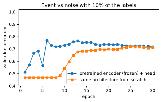
Read the curves from the left. The pretrained encoder is useful from the first epoch: its features already organize the data, so the head reaches its plateau almost immediately. The from-scratch model spends most of its budget at chance level while it learns convolutional filters from only 96 examples, then climbs and, on this small task, eventually gets close. That trajectory is the point: with pretraining you pay for feature learning once, with unlabeled data, instead of paying for it again with every scarce-label task. Exact numbers vary run to run; the early-epoch gap widens as labels get scarcer or models get bigger. Try 5% or 2% of the labels on your own machine.
This is the practical argument for self-supervised learning. Reconstruction, denoising, and masking objectives extract structure from unlabeled data, and unlabeled data is what the geosciences have in abundance. The expensive resource, expert labels, is then spent only on a small labeled set, either through a linear probe as here or through full fine-tuning that also updates the encoder. When you read about foundation models pretrained on continuous seismic archives or satellite-image stacks, this two-stage recipe, self-supervised pretraining followed by light supervised adaptation, is what is meant.
6.1 Does the encoder survive real data? A miniPNW transfer probe
The probe above is synthetic-to-synthetic: an encoder pretrained on synthetic spectrograms, probed with synthetic labels, scored on synthetic validation data. Chapter 4.3 showed what happens when a synthetic-trained classifier meets real waveforms — it collapses to chance. The self-supervised question is subtler and more hopeful: even if the classifier dies, do the pretrained features carry anything across the gap?
The test: build real spectrograms from the labeled miniPNW waveforms cached by Chapter 2.11 (Ni et al., 2023) — 300 real earthquake windows (P pick 7 s into a 30 s window) and 300 pre-event noise windows, each normalized to unit peak like the synthetic waveforms, then run through the identical spectrogram pipeline with the identical global normalization. Then train the identical linear probe — the frozen synthetic-pretrained encoder plus a fresh head — on 96 real labeled examples, the same 10% label budget as before, and evaluate on a held-out test set of real windows. The synthetic-to-synthetic accuracy sits next to the result for direct comparison.
import urllib.request
import h5py
import pandas as pd

# Same files and loader pattern as notebook 2.11, which caches them in its data/ folder
pnw_dir = os.path.join('..', 'Chapter2-DataManipulation', 'data')
os.makedirs(pnw_dir, exist_ok=True)
metadata_path = os.path.join(pnw_dir, 'miniPNW_metadata.csv')
waveform_path = os.path.join(pnw_dir, 'miniPNW_waveforms.hdf5')
base_url = 'https://dasway.ess.washington.edu/shared/niyiyu/PNW-ML'

have_pnw = True
try:
    if not os.path.exists(metadata_path):
        urllib.request.urlretrieve(f'{base_url}/miniPNW_metadata.csv', metadata_path)
    if not os.path.exists(waveform_path):
        print('Downloading miniPNW waveforms (about 670 MB, one-time; shared with notebook 2.11)...')
        urllib.request.urlretrieve(f'{base_url}/miniPNW_waveforms.hdf5', waveform_path)
except Exception as err:
    have_pnw = False
    print('miniPNW cache is missing and the download failed, so the transfer probe below is skipped.\n'
          'Run notebook 2.11 first (it downloads and caches the files), then rerun this section.\n'
          f'Reason: {err!r}')
have_pnw = have_pnw and os.path.exists(waveform_path)
print('miniPNW available:', have_pnw)
miniPNW available: True
if have_pnw:
    meta = pd.read_csv(metadata_path)
    eq = meta[(meta['source_type'] == 'earthquake') & meta['trace_P_arrival_sample'].notna()].copy()
    n_win, pre = 3000, 700  # 30 s at 100 Hz, P pick 7 s into the window
    p_samp = eq['trace_P_arrival_sample'].astype(int)
    eq = eq[(p_samp - pre >= n_win) & (p_samp - pre + n_win <= 15001)].head(300)

    def read_z(f, trace_name):
        """Vertical component of one miniPNW trace (same reader as notebook 2.11)."""
        bucket, narray = trace_name.split('$')
        x, _, z = (int(v) for v in narray.split(',:'))
        return f['/data/' + bucket][x, 2, :z]  # channel order N, E, Z

    R_ev = np.zeros((len(eq), n_win))
    R_no = np.zeros((len(eq), n_win))
    with h5py.File(waveform_path, 'r') as f:
        for i, (_, row) in enumerate(eq.iterrows()):
            tr = read_z(f, row['trace_name']).astype(np.float64)
            pk = int(row['trace_P_arrival_sample'])
            R_ev[i] = tr[pk - pre : pk - pre + n_win]
            R_no[i] = tr[:n_win]  # the trace starts 50 s before the pick: pre-event noise

    R_wave = np.concatenate([R_ev, R_no])
    yR = np.concatenate([np.ones(len(R_ev)), np.zeros(len(R_no))]).astype(int)
    alive = R_wave.std(axis=1) > 0
    R_wave, yR = R_wave[alive], yR[alive]
    R_wave = R_wave - R_wave.mean(axis=1, keepdims=True)
    R_wave = R_wave / np.abs(R_wave).max(axis=1, keepdims=True)  # unit peak, like the synthetics

    # identical spectrogram pipeline, identical global normalization constants
    R_spec = np.stack([normalize(log_spectrogram(w)[0]) for w in R_wave])
    perm_r = np.random.default_rng(11).permutation(len(R_spec))
    n_rt = int(0.8 * len(R_spec))
    TR_train = torch.from_numpy(R_spec[perm_r[:n_rt]]).unsqueeze(1)
    TR_val = torch.from_numpy(R_spec[perm_r[n_rt:]]).unsqueeze(1)
    yR_train = torch.from_numpy(yR[perm_r[:n_rt]]).long()
    yR_val = torch.from_numpy(yR[perm_r[n_rt:]]).long()
    print(f"real spectrograms: {len(R_spec)} ({int(yR.sum())} earthquake, {int((1 - yR).sum())} noise)"
          f" | train {len(TR_train)}, val {len(TR_val)}")
real spectrograms: 600 (300 earthquake, 300 noise) | train 480, val 120
if have_pnw:
    # same 10% label budget as the synthetic probe: 96 real labeled examples
    lab_r = torch.randperm(len(TR_train), generator=torch.Generator().manual_seed(3))[:n_lab]
    real_lab_loader = DataLoader(TensorDataset(TR_train[lab_r], yR_train[lab_r]),
                                 batch_size=32, shuffle=True)

    torch.manual_seed(5)
    probe_real = EncoderClassifier(copy.deepcopy(conv_ae.encoder), freeze=True).to(device)
    acc_real = train_classifier(probe_real, real_lab_loader, X_eval=TR_val, y_eval=yR_val)

    # zero-shot for reference: the probe trained on synthetic labels, applied to real data
    probe.eval()
    with torch.no_grad():
        zeroshot = (probe(TR_val.to(device)).argmax(1).cpu() == yR_val).float().mean().item()

    print(f"linear probe on synthetic val (synthetic labels):  {acc_probe[-1]:.3f}")
    print(f"linear probe on real miniPNW val (real labels):    {acc_real[-1]:.3f}")
    print(f"synthetic-to-real transfer gap:                    {acc_probe[-1] - acc_real[-1]:.3f}")
    print(f"zero-shot (synthetic-label probe on real val):     {zeroshot:.3f}")

    plt.figure(figsize=(5.5, 3.5))
    ep = np.arange(1, len(acc_probe) + 1)
    plt.plot(ep, acc_probe, "o-", label="probe on synthetic data")
    plt.plot(ep, acc_real, "s-", label="same encoder, probe on real miniPNW")
    plt.xlabel("epoch"); plt.ylabel("validation accuracy")
    plt.title("Linear probes on the synthetic-pretrained encoder")
    plt.legend(loc="lower right"); plt.ylim(0.4, 1.02)
    plt.grid(alpha=0.3)
    plt.tight_layout(); plt.show()
linear probe on synthetic val (synthetic labels): 0.717
linear probe on real miniPNW val (real labels): 0.908
synthetic-to-real transfer gap: -0.192
zero-shot (synthetic-label probe on real val): 0.642
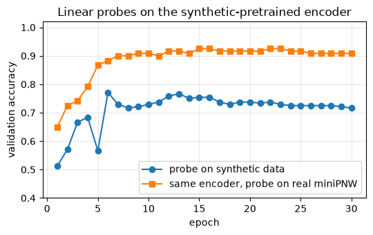
Three numbers to read together, and a sign that may surprise. The synthetic-to-synthetic probe sits at 72.5%. The same frozen encoder, probed with 96 real labels, reaches 90.8% on real miniPNW windows — the transfer “gap” is negative, -18 points. That does not mean synthetic pretraining beats real data; it means the two tasks are not equally hard. The synthetic validation set deliberately includes events down to SNR 0.5, many of them irreducibly undetectable, while miniPNW earthquakes are analyst-picked and mostly clear, and real pre-event noise is spectrally distinctive. The honest conclusions are the relative ones. First, zero-shot fails: the head trained on synthetic labels manages 63.3% on real windows, echoing the collapse of the synthetic-trained classifier in 4.3 — decision boundaries do not transfer. Second, the features underneath do transfer: with not one encoder weight updated on real data, 96 real labels are enough to reach 91%. That asymmetry is the practical case for self-supervised pretraining — representations survive a domain shift that classifiers do not, and the price of crossing it is a hundred labels, not a retrained network.
7. Beyond the bottleneck: skip connections and U-Nets
Our reconstructions are blurry because everything must pass through a low-dimensional bottleneck, which discards fine detail by design. The standard fix is the skip connection: feed the output of each encoder stage directly to the matching decoder stage, so high-resolution detail bypasses the bottleneck while the deep path carries context. An encoder-decoder with skip connections at every level is a U-Net (Ronneberger et al., 2015), the workhorse of image segmentation and of most seismic deep-learning models.
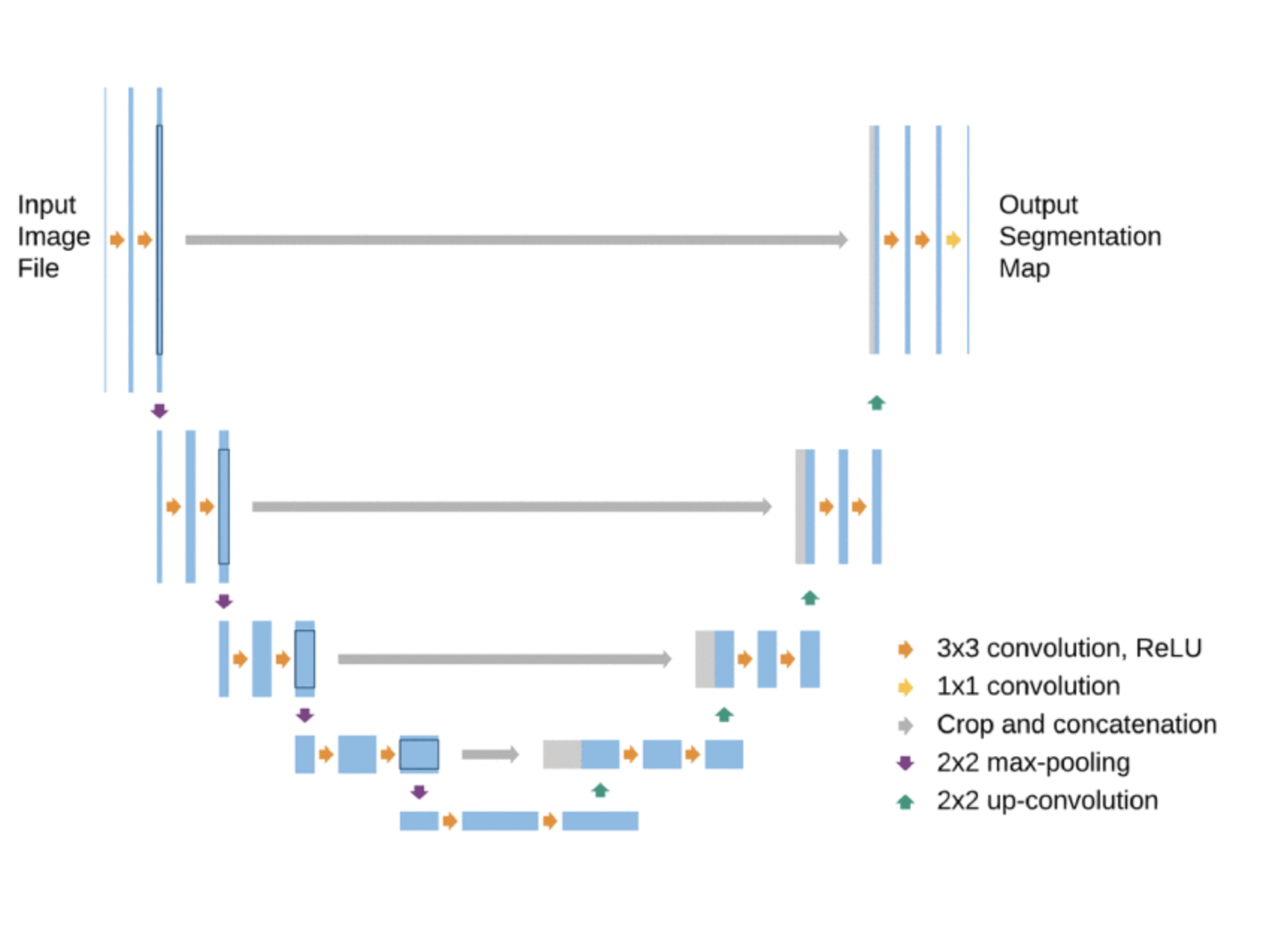
DeepDenoiser and WaveDecompNet from Section 4 both use skip connections, and phase pickers such as PhaseNet are U-Nets applied to waveforms. Multi-task encoder-decoders push the idea further: the Earthquake Transformer (Mousavi et al., 2020) decodes detection, P-pick, and S-pick probabilities from a single encoder. We do not implement U-Nets here; the point is that they are autoencoders plus shortcuts.
Summary
- An autoencoder learns a compact latent representation by reconstructing its own input; no labels needed.
- Convolutional autoencoders beat dense ones on image-like data such as spectrograms.
- Changing the target turns reconstruction into something useful: clean spectrograms give a denoiser (the miniature of DeepDenoiser and WaveDecompNet); reconstructing masked patches gives the objective behind modern masked pretraining.
- The trained encoder is the reusable product: frozen behind a linear probe trained on 10% of the labels, it reached its accuracy plateau within a few epochs, while the same architecture trained from scratch spent most of its budget relearning features.
- The masked objective ported to a second domain — monthly climate-anomaly maps — with no change beyond a new data loader; portability across domains is the point of self-supervision.
- Probed on real miniPNW spectrograms, the frozen synthetic-pretrained encoder supports 90.8% accuracy from 96 real labels, while the synthetic-label head transfers at only 63.3%: features cross the synthetic-to-real gap, decision boundaries do not.
Next: physics-informed neural networks, where the loss function itself encodes the governing equations.
- Ni, Y., Hutko, A., Skene, F., Denolle, M., Malone, S., Bodin, P., Hartog, R., & Wright, A. (2023). Curated Pacific Northwest AI-ready Seismic Dataset. Seismica, 2(1). 10.26443/seismica.v2i1.368