Dense networks treat every input feature as independent. Time series are not: the order of the samples carries the signal. This notebook builds four models that read a sequence, in order of increasing sophistication: a vanilla recurrent network, an LSTM, a single-head self-attention layer written from scratch, and a small Transformer encoder. All four solve the same forecasting task on the same data, so we can compare them directly.
A recurrent neuron receives an input and the output it produced at the previous time step. Because each step reuses the previous step’s output, the network has memory. Simple recurrent cells have short memory, on the order of tens of steps; much of this notebook is about doing better.
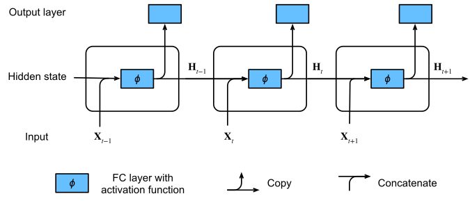
From Dive into Deep Learning: an RNN with a hidden state. At each time step the cell combines the current input with the hidden state from the previous step.
import time

import numpy as np
import pandas as pd
import matplotlib.pyplot as plt
import torch

import mlgeo_synth

torch.manual_seed(42)
np.random.seed(42)

device = torch.device("cuda" if torch.cuda.is_available()
                      else "mps" if torch.backends.mps.is_available()
                      else "cpu")
print(f"Detected device: {device}")

# The models in this notebook are tiny, and recurrent layers launch one small
# operation per time step, so accelerator overhead dominates any speedup.
# CPU is usually fastest for models this size.
device = torch.device("cpu")
print(f"Using device: {device}")
Detected device: cpu
Using device: cpu
1. Forecasting vocabulary
In time series forecasting, the goal is to predict future values from historical data. Two definitions come up constantly:
- Context window (also called look-back window or input window): the stretch of past data the model reads before making a prediction. Its length sets how much history the model can use to pick up trends and seasonality.
- Forecast horizon (also called prediction length): the number of future time steps the model predicts. A horizon of 30 means the model outputs the next 30 values in one shot.
We will use a context window of 90 days and a forecast horizon of 30 days.
2. Data: a synthetic GNSS displacement series
GNSS stations record ground position to millimeter precision, day after day, for decades. A displacement time series at one station mixes several physical signals: steady tectonic motion, seasonal loading from water and snow, sudden coseismic offsets when an earthquake happens, and slow postseismic relaxation afterward, all on top of instrument and environment noise.
The mlgeo_synth package generates such a series with known components, so we can see exactly what the models are asked to forecast. We generate 10 years of daily displacement in millimeters, with an earthquake placed near the middle of the record.
eq_day = 1800  # earthquake day, near the middle of the 10-year record
gnss = mlgeo_synth.gnss_series(n_years=10.0, eq_day=eq_day, seed=42)
print(f"{len(gnss)} daily samples, columns: {list(gnss.columns)}")
gnss.head()
3652 daily samples, columns: ['date', 'disp_mm', 'trend_mm', 'seasonal_mm', 'eq_mm']
fig, axes = plt.subplots(2, 1, figsize=(8, 5), sharex=True)

axes[0].plot(gnss["date"], gnss["disp_mm"], color="#333333", lw=0.6,
             label="disp_mm (observed)")
axes[0].set_ylabel("displacement (mm)")
axes[0].legend(loc="upper left")
axes[0].grid(alpha=0.3)

axes[1].plot(gnss["date"], gnss["trend_mm"], color="#4477AA", label="trend_mm")
axes[1].plot(gnss["date"], gnss["seasonal_mm"], color="#CCBB44", label="seasonal_mm")
axes[1].plot(gnss["date"], gnss["eq_mm"], color="#EE6677", label="eq_mm")
axes[1].set_ylabel("component (mm)")
axes[1].set_xlabel("date")
axes[1].legend(loc="upper left")
axes[1].grid(alpha=0.3)

plt.tight_layout()
plt.show()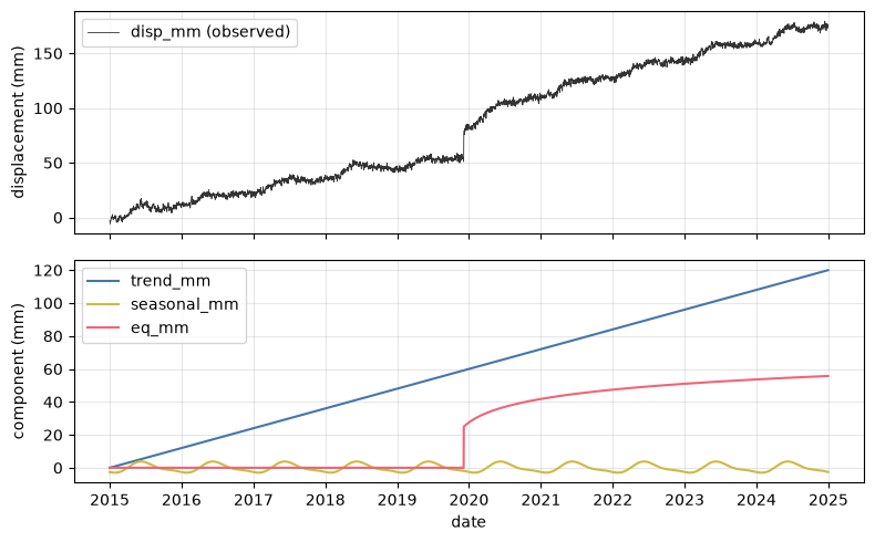
The earthquake step and the curved postseismic recovery sit on top of a steady trend of about 12 mm/yr and a few-millimeter seasonal cycle. The forecasting task: given the last 90 days of displacement, predict the next 30 days.
3. Supervised pairs and a temporal split
Four preprocessing rules for sequence forecasting:
- Standardize the series (subtract the mean, divide by the standard deviation) so the network trains on values near zero. Compute the statistics on the training portion only, then apply them everywhere.
- Slide a window over the series to build (input, target) pairs: 90 days of context as input, the following 30 days as target.
- Split in time, not at random. The first 8 years become training data, the last 2 years validation. No window crosses the split boundary, and no data is shuffled across it. Shuffling windows within the training set during training is fine.
- Anchor each window. Subtract the last context value from both the context and the target, so the model forecasts change relative to the most recent observation. This series trends upward for 10 years, so validation windows sit at absolute levels the training set never contained; without anchoring, every model would have to extrapolate outside its training range and the saturating ones (tanh, sigmoid) would fail badly. Try removing the anchor later and watch the validation errors grow.
A random split would leak information: a “validation” window could overlap almost entirely with two training windows on either side of it, and the validation score would say nothing about forecasting genuinely unseen time.
WINDOW, HORIZON = 90, 30

series = gnss["disp_mm"].to_numpy(dtype=np.float32)
n_days = len(series)
split = int(0.8 * n_days)  # first 8 years train, last 2 years validation

mu = float(series[:split].mean())
sigma = float(series[:split].std())
z = (series - mu) / sigma
print(f"training-portion mean {mu:.1f} mm, std {sigma:.1f} mm")


def make_windows(z, start, stop, window=WINDOW, horizon=HORIZON):
    """Build anchored (window, horizon) pairs from z[start:stop]."""
    X, Y = [], []
    for i in range(start, stop - window - horizon + 1):
        X.append(z[i : i + window])
        Y.append(z[i + window : i + window + horizon])
    X = np.stack(X)[..., np.newaxis]      # (n_pairs, window, 1)
    Y = np.stack(Y)                       # (n_pairs, horizon)
    anchor = X[:, -1:, 0].copy()          # last context value, (n_pairs, 1)
    X = X - anchor[:, :, np.newaxis]      # context relative to its last day
    Y = Y - anchor                        # target relative to the same day
    return (torch.from_numpy(X), torch.from_numpy(Y),
            torch.from_numpy(anchor))


X_train, Y_train, anc_train = make_windows(z, 0, split)
X_val, Y_val, anc_val = make_windows(z, split, n_days)
print("train:", tuple(X_train.shape), "->", tuple(Y_train.shape))
print("val:  ", tuple(X_val.shape), "->", tuple(Y_val.shape))
training-portion mean 64.4 mm, std 46.6 mm
train: (2802, 90, 1) -> (2802, 30)
val: (612, 90, 1) -> (612, 30)
i = 300  # one validation pair, shown in original units
a = anc_val[i].item()
ctx_mm = (X_val[i, :, 0].numpy() + a) * sigma + mu
tgt_mm = (Y_val[i].numpy() + a) * sigma + mu

plt.figure(figsize=(6, 3))
plt.plot(np.arange(WINDOW), ctx_mm, color="#4477AA", label="context (90 days)")
plt.plot(np.arange(WINDOW, WINDOW + HORIZON), tgt_mm, color="#EE6677",
         label="target (30 days)")
plt.axvline(WINDOW, color="gray", lw=0.8, ls="--")
plt.xlabel("day within window")
plt.ylabel("displacement (mm)")
plt.legend()
plt.grid(alpha=0.3)
plt.tight_layout()
plt.show()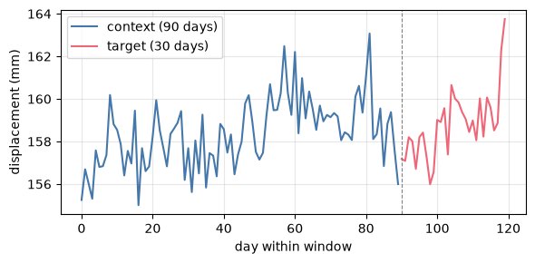
4. One training loop, one metric
Every model below maps a (90, 1) context to 30 forecast values. To keep the comparison fair, they all share the same windows, the same loss (MSE on standardized values), the same optimizer settings, and the same validation metric: mean absolute error over the 30-day horizon, converted back to millimeters.
Training runs for 20 epochs, enough for models this small. Raise the epoch count on your own machine if you want tighter convergence.
results = {}


def count_params(model):
    return sum(p.numel() for p in model.parameters())


def val_mae_mm(model):
    """Mean absolute error on the validation windows, in millimeters."""
    model.eval()
    with torch.no_grad():
        pred = model(X_val.to(device)).cpu()
    return (pred - Y_val).abs().mean().item() * sigma


def train_model(model, name, n_epochs=20, lr=1e-3, batch_size=64):
    model = model.to(device)
    opt = torch.optim.Adam(model.parameters(), lr=lr)
    loss_fn = torch.nn.MSELoss()
    n = X_train.shape[0]
    history = {"train": [], "val": []}
    t0 = time.time()
    for epoch in range(n_epochs):
        model.train()
        perm = torch.randperm(n)  # shuffle within the training set only
        running = 0.0
        for j in range(0, n, batch_size):
            idx = perm[j : j + batch_size]
            xb, yb = X_train[idx].to(device), Y_train[idx].to(device)
            opt.zero_grad()
            loss = loss_fn(model(xb), yb)
            loss.backward()
            opt.step()
            running += loss.item() * len(idx)
        history["train"].append(running / n)
        model.eval()
        with torch.no_grad():
            val_loss = loss_fn(model(X_val.to(device)), Y_val.to(device)).item()
        history["val"].append(val_loss)
        if (epoch + 1) % 5 == 0:
            print(f"[{name}] epoch {epoch + 1:2d}  "
                  f"train MSE {history['train'][-1]:.4f}  val MSE {val_loss:.4f}")
    elapsed = time.time() - t0
    mae = val_mae_mm(model)
    results[name] = {"model": model, "history": history,
                     "n_params": count_params(model),
                     "train_time_s": elapsed, "val_mae_mm": mae}
    print(f"[{name}] {count_params(model):,} parameters, "
          f"trained in {elapsed:.1f} s, val MAE {mae:.2f} mm")
5. Vanilla RNN
torch.nn.RNN implements the simple recurrent cell. At each time step it updates the hidden state as : the new input mixed with the previous hidden state. We read out the hidden state after the last of the 90 steps and map it to 30 forecast values with a linear layer.
class VanillaRNN(torch.nn.Module):
    def __init__(self, hidden_size=32, horizon=HORIZON):
        super().__init__()
        self.rnn = torch.nn.RNN(1, hidden_size, batch_first=True)
        self.head = torch.nn.Linear(hidden_size, horizon)

    def forward(self, x):                # x: (batch, window, 1)
        out, _ = self.rnn(x)             # out: (batch, window, hidden)
        return self.head(out[:, -1, :])  # last hidden state -> 30 values


train_model(VanillaRNN(), "RNN")
[RNN] epoch 5 train MSE 0.0044 val MSE 0.0027
[RNN] epoch 10 train MSE 0.0042 val MSE 0.0025
[RNN] epoch 15 train MSE 0.0042 val MSE 0.0026
[RNN] epoch 20  train MSE 0.0042  val MSE 0.0025
[RNN] 2,110 parameters, trained in 5.8 s, val MAE 1.83 mm
hist = results["RNN"]["history"]
plt.figure(figsize=(6, 3))
plt.plot(hist["train"], color="#4477AA", label="train")
plt.plot(hist["val"], color="#EE6677", label="validation")
plt.yscale("log")
plt.xlabel("epoch")
plt.ylabel("MSE (standardized units)")
plt.title("Vanilla RNN learning curves")
plt.legend()
plt.grid(alpha=0.3)
plt.tight_layout()
plt.show()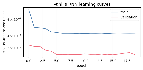
6. Why plain RNNs forget: vanishing and exploding gradients
Training a recurrent network uses backpropagation through time (BPTT): unroll the network over the 90 time steps, then push the gradient of the loss backward through every step. The gradient that reaches step 1 is a product of roughly 90 Jacobian matrices, one per step. Multiply 90 numbers slightly smaller than one and the product is nearly zero; multiply 90 numbers slightly larger than one and it explodes. Matrix products behave the same way: repeated multiplication shrinks or blows up exponentially with sequence length.
When the product shrinks, which is the common case with tanh cells, the early time steps receive almost no gradient. The network cannot learn that something 80 days back matters for the forecast, because the training signal never reaches that far into the past. This is the vanishing gradient problem, and it is the reason simple recurrent memory tops out around a few tens of steps. When the product grows instead, training becomes unstable; gradient clipping keeps that case under control, but there is no equally simple fix for vanishing.
Two families of fixes changed the field. The LSTM (1997) adds a gated memory cell whose state is updated by addition rather than repeated multiplication, giving gradients a path that does not shrink. Attention, introduced by Bahdanau et al. (2014) as an add-on to recurrent sequence-to-sequence models, lets every time step connect directly to every other; the Transformer (Vaswani et al., 2017, “Attention is all you need”) then removed the recurrence entirely, so no gradient has to survive a 90-step product. We build both next.
7. LSTM
The Long Short-Term Memory cell carries an internal cell state alongside the hidden state and controls it with three learned gates. The forget gate decides how much of the previous cell state to keep, the input gate decides how much new candidate information to write into it, and the output gate decides how much of the cell state to expose as the hidden state. Because the cell state is updated by addition, gradients can cross many time steps without vanishing. The price is about four times the parameters of a plain RNN cell of the same width.
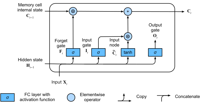
Swapping nn.RNN for nn.LSTM is a one-line change; the rest of the model and the training call are identical.
class LSTMForecaster(torch.nn.Module):
    def __init__(self, hidden_size=32, horizon=HORIZON):
        super().__init__()
        self.lstm = torch.nn.LSTM(1, hidden_size, batch_first=True)
        self.head = torch.nn.Linear(hidden_size, horizon)

    def forward(self, x):
        out, _ = self.lstm(x)
        return self.head(out[:, -1, :])


train_model(LSTMForecaster(), "LSTM")
[LSTM] epoch 5 train MSE 0.0047 val MSE 0.0028
[LSTM] epoch 10 train MSE 0.0042 val MSE 0.0025
[LSTM] epoch 15 train MSE 0.0042 val MSE 0.0025
[LSTM] epoch 20  train MSE 0.0042  val MSE 0.0026
[LSTM] 5,470 parameters, trained in 4.7 s, val MAE 1.86 mm
8. Self-attention from scratch
Attention takes a different route: drop the recurrence and let every time step look directly at every other one. Each position in the window emits a query (“what am I looking for?”), a key (“what do I contain?”), and a value (“what do I pass along?”). The output at each position is a weighted average of all the values, with weights set by how well that position’s query matches every key. One attention head fits in about 15 lines of PyTorch.
class TinyAttention(torch.nn.Module):
    def __init__(self, d_model=32, horizon=HORIZON):
        super().__init__()
        self.embed = torch.nn.Linear(1, d_model)  # lift each scalar to a vector
        self.Wq = torch.nn.Linear(d_model, d_model, bias=False)
        self.Wk = torch.nn.Linear(d_model, d_model, bias=False)
        self.Wv = torch.nn.Linear(d_model, d_model, bias=False)
        self.head = torch.nn.Linear(d_model, horizon)
        self.scale = d_model ** 0.5

    def forward(self, x):                              # x: (batch, window, 1)
        h = self.embed(x)                              # (batch, window, d_model)
        Q, K, V = self.Wq(h), self.Wk(h), self.Wv(h)   # three views of h
        scores = Q @ K.transpose(1, 2) / self.scale    # (batch, window, window)
        weights = torch.softmax(scores, dim=-1)        # rows sum to one
        context = weights @ V                          # weighted sum of values
        return self.head(context.mean(dim=1))          # mean-pool, then forecast
Line by line:
self.embedlifts each scalar displacement to ad_model-dimensional vector; attention operates on vectors, not scalars.Wq,Wk,Wvare three linear maps that produce the queriesQ, keysK, and valuesV, each of shape (batch, 90,d_model). They are three learned “views” of the same embedded sequence.Q @ K.transpose(1, 2)computes all query-key dot products at once: a 90-by-90 score matrix per sample. Entry measures how relevant day is to day .- Dividing by keeps the scores near unit scale so the softmax does not saturate.
softmax(scores, dim=-1)turns each row of scores into positive weights that sum to one.weights @ Vforms the weighted average: each day’s output mixes information from all 90 days, near or far, at the same cost. No 90-step product of Jacobians anywhere.- We mean-pool over the 90 positions and apply a linear head to produce the 30 forecast values.
Note what is missing: nothing in these lines knows the order of the time steps. Shuffle the 90 days of a window and the mean-pooled output is identical. The Transformer fixes this with positional encodings.
train_model(TinyAttention(), "Attention")[Attention] epoch 5 train MSE 0.0047 val MSE 0.0028
[Attention] epoch 10 train MSE 0.0045 val MSE 0.0026
[Attention] epoch 15 train MSE 0.0045 val MSE 0.0026
[Attention] epoch 20  train MSE 0.0045  val MSE 0.0026
[Attention] 4,126 parameters, trained in 4.4 s, val MAE 1.87 mm
9. Transformer encoder
A Transformer encoder layer is self-attention plus a small feed-forward network, with residual connections and layer normalization around each, and usually several attention heads in parallel. PyTorch ships the whole block as torch.nn.TransformerEncoderLayer; we stack two of them with torch.nn.TransformerEncoder.
Because attention is order-blind, we first add a positional encoding to the embedded inputs: a fixed pattern of sines and cosines at different frequencies, one vector per position. After this addition, day 3 and day 73 of a window look different to the model even when their displacement values are equal.
class PositionalEncoding(torch.nn.Module):
    def __init__(self, d_model, max_len=500):
        super().__init__()
        pos = torch.arange(max_len).unsqueeze(1).float()
        freq = torch.exp(torch.arange(0, d_model, 2).float()
                         * (-np.log(10000.0) / d_model))
        pe = torch.zeros(max_len, d_model)
        pe[:, 0::2] = torch.sin(pos * freq)
        pe[:, 1::2] = torch.cos(pos * freq)
        self.register_buffer("pe", pe)

    def forward(self, x):                 # x: (batch, seq, d_model)
        return x + self.pe[: x.shape[1]]


class TinyTransformer(torch.nn.Module):
    def __init__(self, d_model=32, nhead=4, num_layers=2, horizon=HORIZON):
        super().__init__()
        self.embed = torch.nn.Linear(1, d_model)
        self.pos = PositionalEncoding(d_model)
        layer = torch.nn.TransformerEncoderLayer(
            d_model=d_model, nhead=nhead, dim_feedforward=64,
            dropout=0.0, batch_first=True)
        self.encoder = torch.nn.TransformerEncoder(
            layer, num_layers=num_layers, enable_nested_tensor=False)
        self.head = torch.nn.Linear(d_model, horizon)

    def forward(self, x):
        h = self.encoder(self.pos(self.embed(x)))
        return self.head(h.mean(dim=1))


train_model(TinyTransformer(), "Transformer")
[Transformer] epoch 5 train MSE 0.0049 val MSE 0.0031
[Transformer] epoch 10 train MSE 0.0049 val MSE 0.0031
[Transformer] epoch 15 train MSE 0.0046 val MSE 0.0027
[Transformer] epoch 20  train MSE 0.0042  val MSE 0.0025
[Transformer] 18,142 parameters, trained in 29.6 s, val MAE 1.84 mm
10. Comparison
All four models were trained on the same windows and scored with the same metric, so the numbers below are directly comparable. The table also carries two rows that cost nothing to train:
- Persistence: every day of the forecast equals the last day of the context. In our anchored coordinates that forecast is exactly zero, so its MAE is one line of code.
- Seasonal naive: every forecast day equals the observed value 365 days earlier — the right baseline for a purely seasonal series.
A learned forecaster that does not beat persistence has learned nothing; that is the reading rule for every architecture row below.
# Baselines that require no training
# persistence: in anchored coordinates the forecast is identically zero
mae_persistence = Y_val.abs().mean().item() * sigma

# seasonal naive: each forecast day equals the value 365 days earlier
starts = np.arange(split, n_days - WINDOW - HORIZON + 1)  # anchor day of each validation pair
seas_pred = np.stack([z[i + WINDOW - 365 : i + WINDOW + HORIZON - 365] for i in starts])
true_z = Y_val.numpy() + anc_val.numpy()                  # targets back in absolute z units
mae_seasonal = float(np.abs(seas_pred - true_z).mean() * sigma)

baseline_rows = [
    {"model": "persistence (last value)", "parameters": 0, "train time (s)": 0.0,
     "val MAE, 30-day horizon (mm)": round(mae_persistence, 2)},
    {"model": "seasonal naive (365 d earlier)", "parameters": 0, "train time (s)": 0.0,
     "val MAE, 30-day horizon (mm)": round(mae_seasonal, 2)},
]
comparison = pd.DataFrame(
    baseline_rows +
    [{"model": name,
      "parameters": r["n_params"],
      "train time (s)": round(r["train_time_s"], 1),
      "val MAE, 30-day horizon (mm)": round(r["val_mae_mm"], 2)}
     for name, r in results.items()]
).set_index("model")
comparisonmodel_colors = {"RNN": "#4477AA", "LSTM": "#EE6677",
"Attention": "#228833", "Transformer": "#AA3377"}
fig, axes = plt.subplots(1, 2, figsize=(10, 3.5))
for name, r in results.items():
axes[0].plot(r["history"]["val"], color=model_colors[name], label=name)
axes[0].set_yscale("log")
axes[0].set_xlabel("epoch")
axes[0].set_ylabel("validation MSE (standardized units)")
axes[0].set_title("Validation loss")
axes[0].legend()
axes[0].grid(alpha=0.3)
i = 300 # same validation window as before
a = anc_val[i].item()
t_ctx = np.arange(WINDOW)
t_fut = np.arange(WINDOW, WINDOW + HORIZON)
axes[1].plot(t_ctx, (X_val[i, :, 0].numpy() + a) * sigma + mu,
color="#333333", lw=1, label="context")
axes[1].plot(t_fut, (Y_val[i].numpy() + a) * sigma + mu,
color="#333333", lw=2, ls="--", label="truth")
for name, r in results.items():
r["model"].eval()
with torch.no_grad():
pred = r["model"](X_val[i : i + 1].to(device)).cpu().numpy()[0]
axes[1].plot(t_fut, (pred + a) * sigma + mu, color=model_colors[name],
lw=1.2, label=name)
axes[1].set_xlabel("day within window")
axes[1].set_ylabel("displacement (mm)")
axes[1].set_title("One validation forecast")
axes[1].legend(fontsize=8)
axes[1].grid(alpha=0.3)
plt.tight_layout()
plt.show()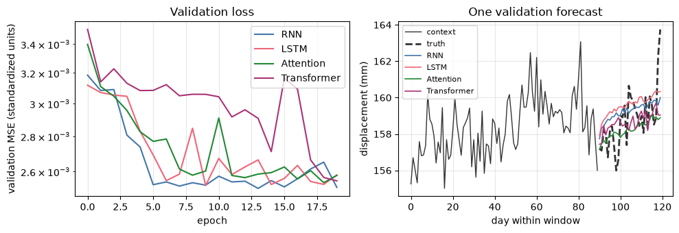
Start with the baseline rows. Persistence scores 2.10 mm, and the four learned models land at 1.83-1.87 mm: an improvement of about 13%, real but modest, which is the correct headline for a series this dominated by smooth trend and seasonality. Seasonal naive fails at 15.5 mm — the value 365 days earlier is systematically about 12 mm low on a 12 mm/yr tectonic trend — a reminder that a baseline only informs when it matches the structure it targets. The four learned scores sit close together, and that is expected. This synthetic series is dominated by a trend and a seasonal cycle that every architecture can extract from a 90-day context, and 20 epochs on a few thousand windows leaves noise in the ordering; rerun with a different seed and the ranking can shuffle. The ranking is not the lesson. The mechanics are: how each architecture moves information across time, and what that costs in parameters and gradient behavior.
Exercise
Double the forecast horizon to 60 days (set HORIZON = 60, rebuild the windows, retrain all four models). How do the validation MAEs change, and why?
Solution
All four MAEs grow, because uncertainty accumulates with lead time: day 60 depends on noise, seasonal phase, and any transient behavior that the 90-day context constrains less and less. The error is not uniform across the horizon either; if you compute the MAE per lead day, the first days of the forecast are much better than the last. The relative ranking of the four models usually stays within noise on this synthetic series.
11. Summary
- A forecasting task is defined by its context window and forecast horizon; supervised pairs come from sliding that window over the series, with a temporal train/validation split so no information leaks across the boundary.
- A vanilla RNN carries a hidden state through time but cannot learn long-range structure, because BPTT multiplies about one Jacobian per time step and the product vanishes or explodes.
- The LSTM routes information through an additively updated cell state, controlled by forget, input, and output gates, so gradients survive long sequences.
- Self-attention connects every time step to every other in one operation: queries, keys, values, scaled dot products, softmax, weighted sum. A Transformer encoder wraps that in residual connections, layer normalization, and feed-forward blocks, plus positional encodings to restore order information.
Attention is the building block behind current forecasting systems, from machine learning weather models to pretrained time series forecasters. Notebook 4.10 runs a forecasting comparison of these architectures on real geoscience data.