1. Introduction
Physics-Informed Neural Networks (PINNs) build physical laws, expressed as ordinary or partial differential equations (ODEs/PDEs), directly into the training of a neural network. The physics enters through the loss function: in addition to fitting data, the network is penalized when its predictions violate the governing equation. PINNs can:
- solve differential equations with or without data,
- work with few labeled samples, because the physics constrains the solution,
- fold prior knowledge into a machine learning workflow.
Geoscience is full of processes governed by well-known equations: heat diffusion in the crust, seismic wave propagation, groundwater flow (Darcy’s law), and fluid dynamics (Navier-Stokes). PINNs were introduced by Raissi et al. (2019) and reviewed for the broader physics community by Karniadakis et al. (2021); see the References at the end of this notebook. Example uses in geoscience:
- Temperature diffusion in the crust: infer thermal structure and geothermal potential from sparse borehole temperature profiles.
- Seismic wave propagation: solve wave equations in heterogeneous media without meshing the domain.
- Groundwater flow: solve the Darcy and advection-diffusion equations to model aquifer response and pollutant transport.
In all three cases the appeal is the same: field data are sparse and noisy, but the governing PDE is known. The physics fills in where the data cannot.
🖥️ Lecture slides — Session 26 (Wed Dec 2, enrichment context)
2. Mathematical framework
A PINN has three components:
- A neural network with parameters θ that approximates the solution .
- A governing equation written in residual form , where is a differential operator. The derivatives of that appear in are computed exactly with automatic differentiation, the same machinery that backpropagation uses.
- A composite loss function
where
- the data loss measures misfit to observations,
- the physics loss is the mean squared PDE residual evaluated at collocation points sampled inside the domain,
- the initial/boundary condition loss pins the solution where it is known.
Training minimizes the combined loss with a gradient-based optimizer such as Adam. The relative weights of the three terms are hyperparameters, and balancing them is one of the practical difficulties of PINNs (more on this in Section 5).
import functools
import time

import matplotlib.pyplot as plt
import numpy as np
import torch
import torch.nn as nn
import torch.optim as optim

device = torch.device("cuda" if torch.cuda.is_available()
                      else "mps" if torch.backends.mps.is_available()
                      else "cpu")
# PINN training differentiates through gradients (double-backward autograd),
# which is most reliable on CPU, and these models are tiny: we train on CPU.
DEVICE = torch.device("cpu")
torch.set_num_threads(1)  # single thread is fastest for such small tensors

torch.manual_seed(42)
np.random.seed(10)
3. Warm-up: Newton’s law of cooling
Before tackling a PDE, we start with an ODE, where automatic differentiation only needs first derivatives. Consider a rock sample cooling toward the ambient temperature . Newton’s law of cooling states
where is a cooling rate constant. With initial temperature , the analytic solution is
We will run a three-way comparison on the same 10 noisy measurements, all taken early in the cooling history:
- a plain neural network (baseline),
- the same network with L2 weight regularization,
- the same network with a physics loss (a PINN).
The question is which model extrapolates correctly beyond the time range covered by the data.
def cooling_law(time, Tenv, T0, R):
    T = Tenv + (T0 - Tenv) * np.exp(-R * time)
    return T
We generate synthetic noisy data: the true curve spans 1000 s, but the 10 training samples only cover the first 300 s.
Tenv = 25
T0 = 100
R = 0.005
times = np.linspace(0, 1000, 1000)
eq = functools.partial(cooling_law, Tenv=Tenv, T0=T0, R=R)
temps = eq(times)

# Make training data
t = np.linspace(0, 300, 10)
T = eq(t) + 2 * np.random.randn(10)

plt.figure(figsize=(6, 4))
plt.plot(times, temps)
plt.plot(t, T, 'o')
plt.legend(['Equation', 'Training data'])
plt.ylabel('Temperature (C)')
plt.xlabel('Time (s)')
plt.title('Newton cooling: truth and noisy samples')
plt.show()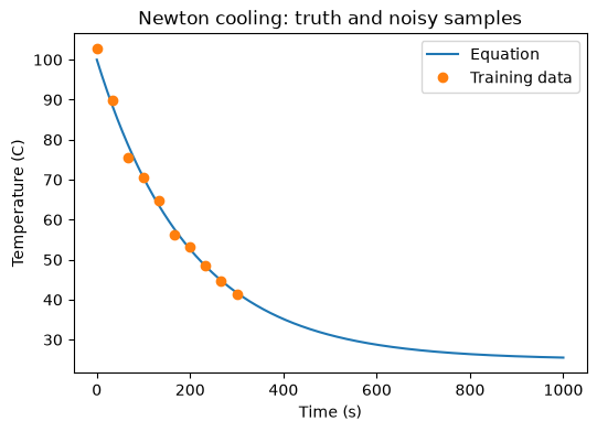
3.1 A network with a pluggable second loss
The Net class below is a small fully connected network. Its fit method minimizes the data misfit plus an optional second loss loss2, weighted by loss2_weight. We will reuse the same class for all three experiments and only swap loss2: None for the baseline, an L2 penalty for the regularized network, and a physics residual for the PINN.
The grad helper computes the derivative of network outputs with respect to inputs using torch.autograd.grad with create_graph=True, so the result can itself be differentiated during backpropagation. This is the core trick of PINNs.
def np_to_th(x):
    """Convert a numpy array to a float32 torch tensor of shape (n, -1)."""
    n_samples = len(x)
    return torch.from_numpy(x).to(torch.float).to(DEVICE).reshape(n_samples, -1)


def grad(outputs, inputs):
    """Partial derivative of outputs with respect to inputs.

    Args:
        outputs: (N, 1) tensor
        inputs: (N, D) tensor
    """
    return torch.autograd.grad(
        outputs, inputs, grad_outputs=torch.ones_like(outputs), create_graph=True
    )


class Net(nn.Module):
    def __init__(
        self,
        input_dim,
        output_dim,
        n_units=100,
        epochs=1000,
        loss=nn.MSELoss(),
        lr=1e-3,
        loss2=None,
        loss2_weight=0.1,
    ) -> None:
        super().__init__()

        self.epochs = epochs
        self.loss = loss
        self.loss2 = loss2
        self.loss2_weight = loss2_weight
        self.lr = lr
        self.n_units = n_units

        self.layers = nn.Sequential(
            nn.Linear(input_dim, self.n_units),
            nn.ReLU(),
            nn.Linear(self.n_units, self.n_units),
            nn.ReLU(),
            nn.Linear(self.n_units, self.n_units),
            nn.ReLU(),
            nn.Linear(self.n_units, self.n_units),
            nn.ReLU(),
        )
        self.out = nn.Linear(self.n_units, output_dim)

    def forward(self, x):
        h = self.layers(x)
        out = self.out(h)
        return out

    def fit(self, X, y):
        Xt = np_to_th(X)
        yt = np_to_th(y)

        optimiser = optim.Adam(self.parameters(), lr=self.lr)
        self.train()
        losses = []
        for ep in range(self.epochs):
            optimiser.zero_grad()
            outputs = self.forward(Xt)
            loss = self.loss(yt, outputs)
            if self.loss2:
                loss += self.loss2_weight * self.loss2(self)
            loss.backward()
            optimiser.step()
            losses.append(loss.item())
            if ep % int(self.epochs / 10) == 0:
                print(f"Epoch {ep}/{self.epochs}, loss: {losses[-1]:.2f}")
        return losses

    def predict(self, X):
        self.eval()
        out = self.forward(np_to_th(X))
        return out.detach().cpu().numpy()
3.2 Baseline network
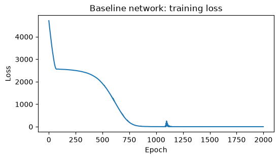
Train on the 10 noisy samples with no extra loss term.
net = Net(1, 1, loss2=None, epochs=2000, lr=1e-4).to(DEVICE)

losses = net.fit(t, T)

plt.figure(figsize=(6, 3))
plt.plot(losses)
plt.xlabel('Epoch')
plt.ylabel('Loss')
plt.title('Baseline network: training loss')
plt.show()
Epoch 0/2000, loss: 4713.87
Epoch 200/2000, loss: 2527.58
Epoch 400/2000, loss: 2299.78
Epoch 600/2000, loss: 1241.00
Epoch 800/2000, loss: 71.03
Epoch 1000/2000, loss: 2.79
Epoch 1200/2000, loss: 1.80
Epoch 1400/2000, loss: 1.52
Epoch 1600/2000, loss: 1.35
Epoch 1800/2000, loss: 1.31
prediction_temp_baseline = net.predict(times)

plt.figure(figsize=(6, 4))
plt.plot(times, prediction_temp_baseline, alpha=0.8)
plt.plot(t, T, 'o')
plt.legend(['Prediction', 'Training data'])
plt.ylabel('Temperature (C)')
plt.xlabel('Time (s)')
plt.title('Baseline network prediction')
plt.show()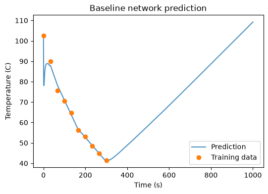
The baseline fits the samples it saw and does whatever it wants after 300 s: nothing constrains the extrapolation.
3.3 L2-regularized network
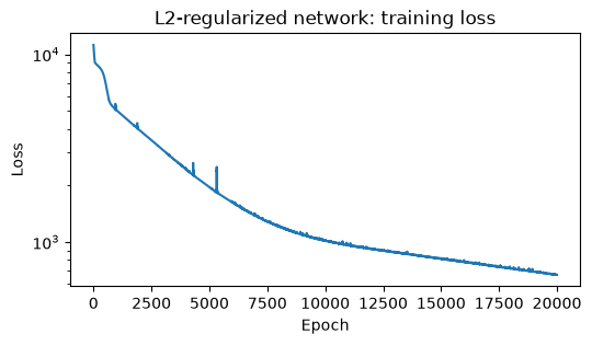
A classic remedy for overfitting is to penalize large weights. We pass the L2 norm of the parameters as loss2.
# Second loss: L2 norm of the network weights
def l2_reg(model: torch.nn.Module):
    return torch.sum(sum([p.pow(2.) for p in model.parameters()]))
netreg = Net(1, 1, loss2=l2_reg, epochs=20000, lr=1e-4, loss2_weight=1).to(DEVICE)
losses = netreg.fit(t, T)
plt.figure(figsize=(6, 3))
plt.plot(losses)
plt.yscale('log')
plt.xlabel('Epoch')
plt.ylabel('Loss')
plt.title('L2-regularized network: training loss')
plt.show()Epoch 0/20000, loss: 11219.99
Epoch 2000/20000, loss: 3925.82
Epoch 4000/20000, loss: 2430.19
Epoch 6000/20000, loss: 1619.53
Epoch 8000/20000, loss: 1206.99
Epoch 10000/20000, loss: 1013.50
Epoch 12000/20000, loss: 920.69
Epoch 14000/20000, loss: 847.17
Epoch 16000/20000, loss: 781.69
Epoch 18000/20000, loss: 722.58
prediction_temp_regularized = netreg.predict(times)

plt.figure(figsize=(6, 4))
plt.plot(times, temps, alpha=0.8)
plt.plot(t, T, 'o')
plt.plot(times, prediction_temp_regularized, alpha=0.8)
plt.plot(times, prediction_temp_baseline, alpha=0.8)
plt.legend(labels=['Equation', 'Training data', 'Regularized', 'Baseline'])
plt.ylabel('Temperature (C)')
plt.xlabel('Time (s)')
plt.title('Baseline vs. L2 regularization')
plt.show()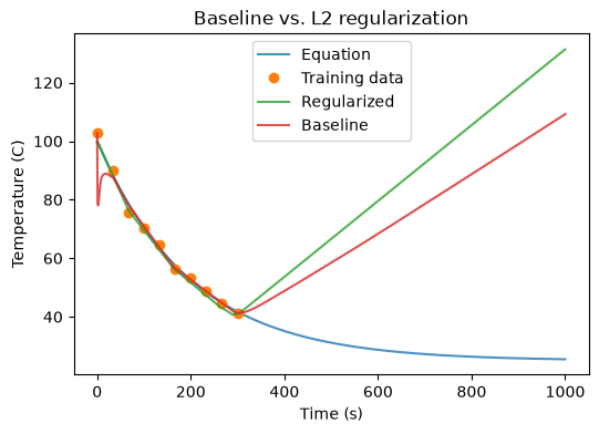
Regularization smooths the prediction, but it has no reason to follow the exponential decay toward : it just keeps the weights small.
3.4 PINN
Now replace the L2 penalty with a physics loss. We evaluate the network at 1000 collocation times spanning the full 1000 s window (far beyond the data), differentiate the output with respect to time using grad, and penalize the mean squared residual of the cooling law
Note that the physics loss uses no temperature observations at all, only the equation.
def physics_loss(model: torch.nn.Module):
    ts = torch.linspace(0, 1000, steps=1000).view(-1, 1).requires_grad_(True).to(DEVICE)
    temps = model(ts)
    dT = grad(temps, ts)[0]
    pde = R * (Tenv - temps) - dT
    return torch.mean(pde**2)
net_PINN = Net(1, 1, loss2=physics_loss, epochs=10000, loss2_weight=1, lr=1e-4).to(DEVICE)
losses = net_PINN.fit(t, T)
plt.figure(figsize=(6, 3))
plt.plot(losses)
plt.yscale('log')
plt.xlabel('Epoch')
plt.ylabel('Loss')
plt.title('PINN: training loss')
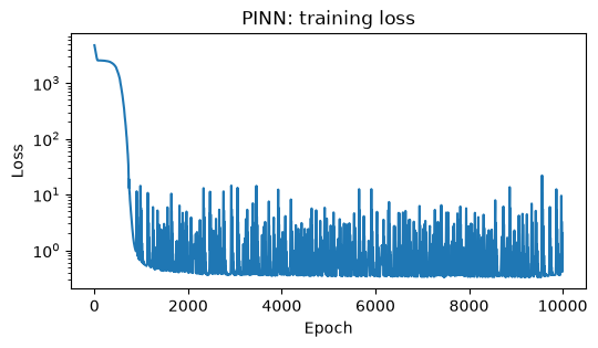
plt.show()Epoch 0/10000, loss: 4775.84
Epoch 1000/10000, loss: 1.88
Epoch 2000/10000, loss: 0.73
Epoch 3000/10000, loss: 0.39
Epoch 4000/10000, loss: 0.36
Epoch 5000/10000, loss: 0.34
Epoch 6000/10000, loss: 0.35
Epoch 7000/10000, loss: 0.34
Epoch 8000/10000, loss: 1.48
Epoch 9000/10000, loss: 1.05
prediction_temp_pinn = net_PINN.predict(times)

plt.figure(figsize=(6, 4))
plt.plot(times, temps, alpha=0.8)
plt.plot(t, T, 'o')
plt.plot(times, prediction_temp_baseline, alpha=0.8)
plt.plot(times, prediction_temp_regularized, alpha=0.8)
plt.plot(times, prediction_temp_pinn, alpha=0.8)
plt.legend(labels=['Equation', 'Training data', 'Baseline', 'Regularized', 'PINN'])
plt.ylabel('Temperature (C)')
plt.xlabel('Time (s)')
plt.title('Three-way comparison')
plt.show()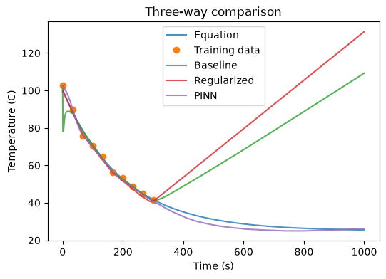
The PINN follows the true exponential decay well past the last data point, because the physics loss constrains the solution everywhere the collocation points reach. The data anchor the amplitude; the equation supplies the shape. That is the whole idea.
Training here is deliberately short. On your own machine you can raise the epoch counts for smoother fits.
4. A real PDE: 1-D heat diffusion in the shallow subsurface
The cooling law was an ODE. Now we solve an actual PDE with a PINN: heat diffusion,
where is temperature and is thermal diffusivity.
Physical setting. Think of a temperature anomaly in the top m of soil or rock, a permafrost active layer or a shallow geothermal profile. A warm anomaly peaks mid-column and relaxes by diffusion, while the surface () and the base () stay pinned at the mean annual temperature, which we take as the 0 °C reference. A typical rock/soil thermal diffusivity is .
Nondimensionalization. Raw SI values (, , in units of 107 s) make ugly numbers for a neural network, so we rescale: and . One unit of corresponds to years; we solve on , roughly one year. Temperature stays in °C. In these units the PDE becomes (diffusivity 1).
Analytic reference. A single sine mode diffuses without changing shape:
with °C. It satisfies the PDE and the boundary conditions at and , so we can measure the PINN’s error exactly.
Network. is a small MLP: 2 inputs, three hidden layers of 64 units, 1 output. We use tanh activations rather than ReLU because the PDE residual needs second derivatives, and the second derivative of ReLU is zero almost everywhere.
T0_heat = 5.0   # amplitude of the initial anomaly, deg C
t_max = 0.3     # nondimensional time horizon (~1 year)


def analytic_T(x, t):
    """Analytic solution: single diffusing sine mode (nondimensional x, t)."""
    return T0_heat * np.sin(np.pi * x) * np.exp(-np.pi**2 * t)


class HeatPINN(nn.Module):
    """T_theta(x, t): 2 inputs -> 3 x 64 tanh -> 1 output."""

    def __init__(self, n_units=64):
        super().__init__()
        self.layers = nn.Sequential(
            nn.Linear(2, n_units), nn.Tanh(),
            nn.Linear(n_units, n_units), nn.Tanh(),
            nn.Linear(n_units, n_units), nn.Tanh(),
            nn.Linear(n_units, 1),
        )

    def forward(self, xt):
        return self.layers(xt)
4.1 Training points
Three sets of points, one per loss term:
- Data points: 40 noisy temperature samples at random locations, like sparse sensor readings, with 0.2 °C Gaussian noise.
- Collocation points: 1000 random interior points where we enforce the PDE residual. No temperature values are attached to them.
- Initial/boundary points: 200 points on the line (initial profile) and 200 on each boundary and (temperature held at 0 °C).
# Data points: sparse noisy samples of the true solution
n_data = 40
x_d = np.random.rand(n_data)
t_d = np.random.rand(n_data) * t_max
T_d = analytic_T(x_d, t_d) + 0.2 * np.random.randn(n_data)
X_data = torch.tensor(np.stack([x_d, t_d], axis=1), dtype=torch.float32)
y_data = torch.tensor(T_d[:, None], dtype=torch.float32)

# Collocation points: interior points where the PDE residual is enforced
n_col = 1000
x_c = torch.rand(n_col, 1)
t_c = torch.rand(n_col, 1) * t_max
X_col = torch.cat([x_c, t_c], dim=1).requires_grad_(True)

# Initial condition points (t = 0) and boundary points (x = 0 and x = 1)
n_b = 200
x_ic = torch.rand(n_b, 1)
X_ic = torch.cat([x_ic, torch.zeros(n_b, 1)], dim=1)
y_ic = T0_heat * torch.sin(np.pi * x_ic)
t_b = torch.rand(n_b, 1) * t_max
X_b0 = torch.cat([torch.zeros(n_b, 1), t_b], dim=1)
X_b1 = torch.cat([torch.ones(n_b, 1), t_b], dim=1)

print(f"data: {X_data.shape}, collocation: {X_col.shape}, "
      f"IC: {X_ic.shape}, BC: {X_b0.shape} + {X_b1.shape}")
data: torch.Size([40, 2]), collocation: torch.Size([1000, 2]), IC: torch.Size([200, 2]), BC: torch.Size([200, 2]) + torch.Size([200, 2])
4.2 Training loop
Each step computes three loss terms and sums them with equal weights:
- Data loss: MSE between and the noisy samples.
- PDE loss: at the collocation points,
gradgives and in one call (columns of the gradient); a secondgradcall on the first column gives . The residual is . - IC/BC loss: MSE against the initial sine profile plus the squared temperature at both boundaries.
A few thousand Adam steps are enough for this smooth problem.
model_heat = HeatPINN().to(DEVICE)
optimizer = optim.Adam(model_heat.parameters(), lr=2e-3)
mse = nn.MSELoss()

n_steps = 2000
history = {"data": [], "pde": [], "icbc": []}

tic = time.perf_counter()
for step in range(n_steps):
    optimizer.zero_grad()

    # Data loss
    loss_data = mse(model_heat(X_data), y_data)

    # PDE residual loss at collocation points
    T_c = model_heat(X_col)
    g = grad(T_c, X_col)[0]           # (n_col, 2): columns are dT/dx, dT/dt
    T_x, T_t = g[:, 0:1], g[:, 1:2]
    T_xx = grad(T_x, X_col)[0][:, 0:1]
    loss_pde = torch.mean((T_t - T_xx) ** 2)

    # Initial and boundary condition loss
    loss_icbc = (mse(model_heat(X_ic), y_ic)
                 + torch.mean(model_heat(X_b0) ** 2)
                 + torch.mean(model_heat(X_b1) ** 2))

    loss = loss_data + loss_pde + loss_icbc
    loss.backward()
    optimizer.step()

    history["data"].append(loss_data.item())
    history["pde"].append(loss_pde.item())
    history["icbc"].append(loss_icbc.item())
    if step % 400 == 0 or step == n_steps - 1:
        print(f"step {step:4d}  data {loss_data.item():.4f}  "
              f"pde {loss_pde.item():.5f}  ic/bc {loss_icbc.item():.5f}")
pinn_train_seconds = time.perf_counter() - tic
print(f"wall-clock training time: {pinn_train_seconds:.1f} s")
step 0 data 2.7585 pde 0.00039 ic/bc 12.18578
step 400 data 0.0477 pde 0.02277 ic/bc 0.01592
step 800 data 0.0425 pde 0.00421 ic/bc 0.00059
step 1200 data 0.0416 pde 0.00915 ic/bc 0.00079
step 1600 data 0.0414 pde 0.01551 ic/bc 0.00082
step 1999  data 0.0413  pde 0.00148  ic/bc 0.00086
wall-clock training time: 15.0 s
4.3 Results
First, predicted vs. analytic temperature profiles at four times. The depth axis is back in meters ().
L = 10.0  # m
x_grid = np.linspace(0, 1, 200)
plot_times = [0.0, 0.05, 0.15, 0.3]
years_per_that = 1e8 / (365.25 * 86400)  # one unit of t_hat in years

plt.figure(figsize=(7, 4.5))
colors = plt.cm.viridis(np.linspace(0, 0.85, len(plot_times)))
for that, c in zip(plot_times, colors):
    X_plot = torch.tensor(np.stack([x_grid, np.full_like(x_grid, that)], axis=1),
                          dtype=torch.float32)
    T_pred = model_heat(X_plot).detach().numpy().ravel()
    label_t = f"t = {that * years_per_that:.2f} yr"
    plt.plot(x_grid * L, analytic_T(x_grid, that), '-', color=c,
             label=f'analytic, {label_t}')
    plt.plot(x_grid * L, T_pred, '--', color=c, label=f'PINN, {label_t}')
plt.xlabel('Depth x (m)')
plt.ylabel('Temperature anomaly (C)')
plt.title('Heat diffusion: PINN vs. analytic solution')
plt.legend(fontsize=8)
plt.show()

# Quantify the error (kept in a dict for the comparison in Section 4.4)
pinn_max_err = {}
for that in plot_times:
    X_plot = torch.tensor(np.stack([x_grid, np.full_like(x_grid, that)], axis=1),
                          dtype=torch.float32)
    T_pred = model_heat(X_plot).detach().numpy().ravel()
    pinn_max_err[that] = np.abs(T_pred - analytic_T(x_grid, that)).max()
    print(f"t_hat = {that:.2f}: max abs error = {pinn_max_err[that]:.3f} C")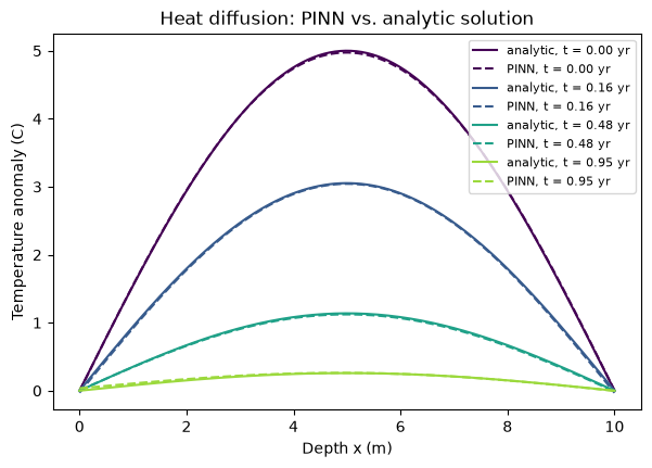
t_hat = 0.00: max abs error = 0.027 C
t_hat = 0.05: max abs error = 0.031 C
t_hat = 0.15: max abs error = 0.016 C
t_hat = 0.30: max abs error = 0.035 C
plt.figure(figsize=(7, 4))
plt.plot(history["data"], label='data loss')
plt.plot(history["pde"], label='PDE residual loss')
plt.plot(history["icbc"], label='IC/BC loss')
plt.yscale('log')
plt.xlabel('Adam iteration')
plt.ylabel('Loss')
plt.title('Loss components during training')
plt.legend()
plt.show()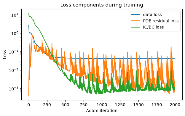
The PINN matches the analytic profiles to a few hundredths of a degree from 40 noisy point measurements, because the PDE and the boundary conditions carry most of the information. The data loss plateaus near the noise floor (the network should not fit the 0.2 °C noise), while the PDE and IC/BC losses drop by three to four orders of magnitude. The periodic spikes in those curves are Adam briefly overshooting and recovering, a common sight in PINN training.
Training is kept short on purpose; on your own machine, raise n_steps and n_col for tighter residuals.
Exercise. Set the PDE loss weight to zero (replace loss_pde with 0 * loss_pde in the sum) and retrain. Compare the profiles at , where there are few data points and the anomaly is small.
Solution
Without the PDE term the model becomes a plain regression on 40 noisy points plus the IC/BC constraints. Near the initial profile, where data are dense relative to the signal, it still looks fine. At later times the predicted profile drifts away from the exponential decay: nothing forces the interior of the domain to behave diffusively, so the network interpolates the noise instead. The error at t_hat = 0.3 typically grows several-fold. This mirrors the cooling-law ablation in Section 3: the physics term is what makes extrapolation trustworthy.
4.4 The baseline: 15 lines of finite differences
This book’s rule is baselines before models, and the physics chapter is not exempt. The forward problem we just solved, with known diffusivity, known initial and boundary conditions, and a smooth solution, is textbook territory for classical numerics, so the PINN has to face the classical method before we praise it. The simplest scheme is FTCS (forward-time, centered-space): put on a grid, replace with the centered second difference, and step forward in time with explicit Euler:
The scheme is only stable for ; we use . That constraint is the price of an explicit method (Crank–Nicolson removes it at the cost of a tridiagonal solve), and on this problem it costs almost nothing. The whole solver, timed:
# FTCS finite differences: the entire solver is the 8 lines between tic and toc
nx = 101
dx = 1.0 / (nx - 1)
dt = 0.4 * dx**2                      # explicit stability requires dt <= dx^2 / 2
nt = int(round(t_max / dt))
x_fd = np.linspace(0.0, 1.0, nx)
r = dt / dx**2
save_steps = {int(round(that / dt)): that for that in plot_times if that > 0}

tic = time.perf_counter()
T_fd = T0_heat * np.sin(np.pi * x_fd)             # initial condition
fd_snapshots = {0.0: T_fd.copy()}
for n in range(1, nt + 1):
    T_fd[1:-1] += r * (T_fd[2:] - 2 * T_fd[1:-1] + T_fd[:-2])
    if n in save_steps:                           # endpoints never updated: T = 0 C
        fd_snapshots[save_steps[n]] = T_fd.copy()
fd_seconds = time.perf_counter() - tic

print(f"FTCS: {nx} grid points, {nt} time steps, "
      f"wall-clock {fd_seconds * 1e3:.0f} ms")
print(f"\n{'t_hat':>6} {'FD max err (C)':>16} {'PINN max err (C)':>18}")
for that in plot_times:
    fd_err = np.abs(fd_snapshots[that] - analytic_T(x_fd, that)).max()
    print(f"{that:6.2f} {fd_err:16.2e} {pinn_max_err[that]:18.3f}")
print(f"\nwall-clock: FD {fd_seconds * 1e3:.0f} ms vs. PINN training "
      f"{pinn_train_seconds:.0f} s -> the PINN is "
      f"{pinn_train_seconds / fd_seconds:.0f}x slower")
FTCS: 101 grid points, 7500 time steps, wall-clock 31 ms
t_hat FD max err (C) PINN max err (C)
0.00 0.00e+00 0.027
0.05 1.73e-04 0.031
0.15 1.94e-04 0.016
0.30 8.83e-05 0.035
wall-clock: FD 31 ms vs. PINN training 15 s -> the PINN is 491x slower
The verdict is not close. The finite-difference solver finishes in about 20 ms and matches the analytic solution to about °C; the PINN needed 14 s of training to get within 0.03 °C. On this forward problem the classical solver wins by a factor of roughly 750 in speed and two orders of magnitude in accuracy, with no learning rate, no architecture, and no seed. That is the honest reading of Section 4.3, and it generalizes: when the coefficients, initial condition, and boundary conditions are known and a standard discretization exists, use the standard discretization. The PINN’s case has to be made elsewhere.
Two things the FD solver did not do, though. It never touched the 40 noisy interior measurements, because a forward solver has no slot for scattered observations. And it required as an input. Both gaps point to the same place, and that is where we go next.
4.5 The inverse problem: recovering the diffusivity
Section 5 will argue that inverse problems are the first regime where PINNs remain the right tool. Here is the demonstration, on the data we already have. Pretend the diffusivity is unknown. In scaled units the generator’s value is exactly , because the nondimensionalization used the true ; the model is not told that. We initialize a trainable at 0.2, five times too low, and let the optimizer recover it from the same 40 noisy samples.
The change to the training loop of Section 4.2 is five lines, marked (1)–(4) below: becomes an nn.Parameter (stored as so it stays positive), it joins the optimizer’s parameter list, and the residual becomes . Everything else is untouched. The information flows like this: the initial condition pins the shape of the anomaly, the 40 samples pin how fast it decays, and the PDE ties that decay rate to .
model_inv = HeatPINN().to(DEVICE)
log_k = nn.Parameter(torch.log(torch.tensor(0.2)))    # (1) trainable k_hat, start 5x too low
optimizer_inv = optim.Adam(list(model_inv.parameters()) + [log_k],  # (2) k joins the optimizer
                           lr=2e-3)

k_history = []
tic = time.perf_counter()
for step in range(n_steps):
    optimizer_inv.zero_grad()
    loss_data = mse(model_inv(X_data), y_data)
    T_c = model_inv(X_col)
    g = grad(T_c, X_col)[0]
    T_x, T_t = g[:, 0:1], g[:, 1:2]
    T_xx = grad(T_x, X_col)[0][:, 0:1]
    loss_pde = torch.mean((T_t - torch.exp(log_k) * T_xx) ** 2)     # (3) k in the residual
    loss_icbc = (mse(model_inv(X_ic), y_ic)
                 + torch.mean(model_inv(X_b0) ** 2)
                 + torch.mean(model_inv(X_b1) ** 2))
    (loss_data + loss_pde + loss_icbc).backward()
    optimizer_inv.step()
    k_history.append(torch.exp(log_k).item())                       # (4) track the estimate
    if step % 400 == 0 or step == n_steps - 1:
        print(f"step {step:4d}  k_hat = {k_history[-1]:.3f}")
inv_seconds = time.perf_counter() - tic

k_rec = k_history[-1]
print(f"\nrecovered k_hat = {k_rec:.3f}  (generator truth 1.0, "
      f"error {abs(k_rec - 1.0) * 100:.1f}%)")
print(f"physical units: k = {k_rec * 1e-6:.2e} m^2/s  (truth 1.00e-06)")
print(f"wall-clock: {inv_seconds:.0f} s")
step 0 k_hat = 0.200
step 400 k_hat = 0.460
step 800 k_hat = 0.733
step 1200 k_hat = 0.880
step 1600 k_hat = 0.949
step 1999  k_hat = 0.982

recovered k_hat = 0.982  (generator truth 1.0, error 1.8%)
physical units: k = 9.82e-07 m^2/s  (truth 1.00e-06)
wall-clock: 16 s
plt.figure(figsize=(6, 3.5))
plt.plot(k_history)
plt.axhline(1.0, color='k', ls=':', label='generator truth')
plt.xlabel('Adam iteration')
plt.ylabel(r'$\hat{k}$ estimate')
plt.title('Diffusivity recovered jointly with the temperature field')
plt.legend()
plt.show()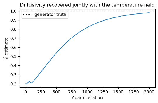
The recovered diffusivity lands within 2% of the generator truth, from 40 noisy point measurements and nothing gridded. Be clear about what this run is: a calibration, also called history matching. The finite-difference solver of Section 4.4 cannot do it alone, because it needs as an input. The classical route wraps the solver in an outer optimization loop that reruns it for every candidate ; in groundwater practice that is what PEST does around a MODFLOW model when calibrating hydraulic conductivity against sparse well records. The PINN merges the two loops: one training run fits the temperature field and inverts for the parameter at the same time, and the same trick extends to many unknowns (a spatially variable can be a second small network). Sparse, noisy point data plus a trusted equation plus unknown coefficients: this is the regime where the extra machinery pays for itself.
4.6 Breaking the PINN: loss-weight imbalance
So far the composite loss has behaved because its three terms happened to sit at comparable scales; equal weights just worked. That is luck, not a law, and Section 5’s warning about loss balancing deserves the same treatment the broken training runs got in notebook 4.5: show the failure, read the symptoms, name the fix.
The exercise in Section 4.3 removed the physics term and watched the model decay into a noisy regression. Here we break the balance in the opposite direction: the physics term swamps the data and initial condition. The run below repeats Section 4.2 with a single change, w_pde = 1e4 on the PDE residual. Watch the printed total: it keeps falling, as if training were going well.
model_bad = HeatPINN().to(DEVICE)
optimizer_bad = optim.Adam(model_bad.parameters(), lr=2e-3)
w_pde = 1e4                       # the only change from Section 4.2

history_bad = {"data": [], "pde": [], "icbc": []}
for step in range(n_steps):
    optimizer_bad.zero_grad()
    loss_data = mse(model_bad(X_data), y_data)
    T_c = model_bad(X_col)
    g = grad(T_c, X_col)[0]
    T_x, T_t = g[:, 0:1], g[:, 1:2]
    T_xx = grad(T_x, X_col)[0][:, 0:1]
    loss_pde = torch.mean((T_t - T_xx) ** 2)
    loss_icbc = (mse(model_bad(X_ic), y_ic)
                 + torch.mean(model_bad(X_b0) ** 2)
                 + torch.mean(model_bad(X_b1) ** 2))
    total = loss_data + w_pde * loss_pde + loss_icbc
    total.backward()
    optimizer_bad.step()
    for key, val in zip(("data", "pde", "icbc"), (loss_data, loss_pde, loss_icbc)):
        history_bad[key].append(val.item())
    if step % 400 == 0 or step == n_steps - 1:
        print(f"step {step:4d}  total {total.item():8.3f}  data {loss_data.item():.3f}  "
              f"pde {loss_pde.item():.5f}  ic/bc {loss_icbc.item():.3f}")
step 0 total 96.174 data 2.569 pde 0.00819 ic/bc 11.750
step 400 total 9.546 data 1.123 pde 0.00000 ic/bc 8.419
step 800 total 9.491 data 1.113 pde 0.00000 ic/bc 8.373
step 1200 total 9.478 data 1.113 pde 0.00000 ic/bc 8.362
step 1600 total 9.491 data 1.116 pde 0.00000 ic/bc 8.371
step 1999 total 9.560 data 1.063 pde 0.00004 ic/bc 8.124
fig, axes = plt.subplots(1, 2, figsize=(11, 4))

axes[0].plot(history_bad["data"], label='data loss')
axes[0].plot(history_bad["pde"], label='PDE residual loss')
axes[0].plot(history_bad["icbc"], label='IC/BC loss')
axes[0].set_yscale('log')
axes[0].set_xlabel('Adam iteration')
axes[0].set_ylabel('Loss (unweighted)')
axes[0].set_title(f'Loss components, w_pde = {w_pde:.0e}')
axes[0].legend()

X_plot0 = torch.tensor(np.stack([x_grid, np.zeros_like(x_grid)], axis=1),
                       dtype=torch.float32)
axes[1].plot(x_grid * L, analytic_T(x_grid, 0.0), 'k-', label='analytic, t = 0')
axes[1].plot(x_grid * L, model_heat(X_plot0).detach().numpy().ravel(), '--',
             label='balanced PINN (Sec. 4.2)')
axes[1].plot(x_grid * L, model_bad(X_plot0).detach().numpy().ravel(), '--',
             label=f'w_pde = {w_pde:.0e}')
axes[1].set_xlabel('Depth x (m)')
axes[1].set_ylabel('Temperature anomaly (C)')
axes[1].set_title('Initial profile: balanced vs. imbalanced')
axes[1].legend()
plt.tight_layout()
plt.show()

err_bad = np.abs(model_bad(X_plot0).detach().numpy().ravel()
                 - analytic_T(x_grid, 0.0)).max()
print(f"max error at t_hat = 0: broken run {err_bad:.2f} C, "
      f"balanced run {pinn_max_err[0.0]:.3f} C  (signal amplitude {T0_heat} C)")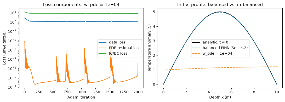
max error at t_hat = 0: broken run 3.86 C, balanced run 0.027 C (signal amplitude 5.0 C)
The total loss falls and the answer is garbage. That combination is the signature of loss imbalance, and it is invisible unless you log the components separately. Read them, not the total: after a few hundred steps the PDE residual is pinned below 10-5, while the data loss sits near 1 (far above the 0.04 noise floor of Section 4.2) and the IC/BC loss stalls near 8, the same order as the 12.5 a network outputting zero everywhere would score (the mean of ). The network has found a near-trivial solution: satisfies the heat equation and the boundary conditions exactly, so the weighted objective rewards staying close to it, and any move toward the true initial profile is punished through the dominant term before it can pay off. The profile at misses the 5 °C anomaly by about 4 °C.
The fix is the balance we already had: with equal weights, the same architecture and the same 2000 steps reached 0.03 °C in Section 4.2. When no fixed weighting works, because the terms have genuinely different scales, the standard moves are to normalize each term by its initial value, tune the weights against a held-out validation metric, or use an adaptive weighting scheme (Karniadakis et al., 2021); longer training and wider layers only help when the imbalance is mild. The habit to take away: always plot the loss components separately. A single total-loss curve hides exactly this failure.
Exercise (spectral bias). The other failure mode Section 5 names is spectral bias. Add a higher-frequency mode to the initial condition:
whose analytic solution adds to the single-mode reference. Regenerate y_ic and the 40 data samples from the two-mode solution, retrain the Section 4.2 PINN (equal weights), and rerun the FTCS solver of Section 4.4 with the new initial profile. Compare both to the analytic solution at .
Solution
The FTCS solver handles the new mode with zero code change: at nx = 101 the seventh mode has about 28 grid points per wavelength. The PINN does not. After the same 2000 steps its initial profile is the smooth first mode with the ripples flattened out: the IC loss stalls near 2 (the mean square of the missing mode, 2^2/2), and the max error at t_hat = 0 is about 2 degrees, the full amplitude of the mode the network refused to learn. That is spectral bias: tanh MLPs fit low frequencies first and high frequencies slowly, if at all. Remedies, in increasing order of effort: train much longer, widen the layers, or give the network Fourier-feature inputs (sin/cos embeddings of x_hat), the standard cure. For diffusion the stakes are low: the seventh mode decays as e^(-49 pi^2 t_hat) and is physically gone within days. For wave equations there is no such mercy, because the high frequencies are the signal.
5. Where PINNs stand in 2026
PINNs are no longer a novelty, and their failure modes are well documented; two of them are now sitting in this notebook. Loss balancing is a persistent tuning problem: a bad balance makes training converge to a solution that satisfies one term and ignores the others, and Section 4.6 showed it on our own problem, where a factor of 104 on the physics term produced a network stuck near the trivial zero solution, missing the 5 °C anomaly by about 4 °C while its total loss kept falling. Standard MLPs also carry a spectral bias toward smooth, low-frequency functions: they learn smooth solutions quickly and oscillatory or fine-scale structure slowly, if at all (Karniadakis et al., 2021); the exercise in 4.6 makes a tanh MLP flatten a seventh-mode ripple that the finite-difference solver resolves without any change. Stiff PDEs, sharp fronts, and widely separated time scales compound both problems, because the residual then varies over orders of magnitude across the domain and no fixed weighting is right everywhere.
The first rule of use is negative: do not solve a clean forward problem with a PINN. Section 4.4 put numbers on this. Fifteen lines of FTCS beat the trained PINN by a factor of roughly 750 in wall-clock time and two orders of magnitude in accuracy, with no hyperparameters to tune. When the coefficients and boundary conditions are known and a standard discretization exists, the classical solver wins. And for the adjacent problem of building fast surrogates evaluated many times, neural operators have largely taken over: the Fourier Neural Operator (Li et al., 2021) and DeepONet (Lu et al., 2021) learn the solution operator, the map from an initial condition, boundary condition, or coefficient field to the solution, so that after training on many simulation pairs a new case costs milliseconds, where a PINN would retrain from scratch. For parametric studies, uncertainty quantification, and operational forecasting, that is the tool that gets used.
PINNs still earn their keep in two regimes, and both are now demonstrated rather than claimed. The first is inverse problems: Section 4.5 made the diffusivity a trainable parameter and recovered it to within 2% from the 40 noisy samples, the PDE acting as the forward model inside a regression (Raissi et al., 2019). This is joint inversion, the PEST-around-MODFLOW pattern of groundwater calibration collapsed into a single training loop. The second is the sparse-data regime those same 40 points represent: scattered, noisy observations plus a trusted governing equation and no simulation library to train an operator on. A forward solver has no slot for such data; the PINN treats them as one more loss term. Both situations are common in geoscience, which is why the method remains part of the toolkit (Karniadakis et al., 2021).
References
- Raissi, M., Perdikaris, P., and Karniadakis, G. E. (2019). Physics-informed neural networks: A deep learning framework for solving forward and inverse problems involving nonlinear partial differential equations. Journal of Computational Physics, 378, 686-707.
- Karniadakis, G. E., Kevrekidis, I. G., Lu, L., Perdikaris, P., Wang, S., and Yang, L. (2021). Physics-informed machine learning. Nature Reviews Physics, 3, 422-440.
- Li, Z., Kovachki, N., Azizzadenesheli, K., Liu, B., Bhattacharya, K., Stuart, A., and Anandkumar, A. (2021). Fourier neural operator for parametric partial differential equations. International Conference on Learning Representations (ICLR).
- Lu, L., Jin, P., Pang, G., Zhang, Z., and Karniadakis, G. E. (2021). Learning nonlinear operators via DeepONet based on the universal approximation theorem of operators. Nature Machine Intelligence, 3, 218-229.
Summary
- A PINN adds the residual of a governing equation, evaluated by automatic differentiation at collocation points, to the training loss.
- On the cooling-law ablation, only the physics term produced correct extrapolation beyond the data; L2 regularization did not.
- On the 1-D heat equation, a 3-layer tanh MLP recovered the analytic diffusing mode from 40 noisy samples plus the PDE and boundary conditions.
- The classical baseline won the forward problem outright: 15 lines of FTCS were a factor of ~750 faster and two orders of magnitude more accurate than the PINN (Section 4.4).
- Making the diffusivity a trainable parameter turned the same loop into a joint inversion that recovered to within 2% from the 40 noisy samples, a calibration the forward solver cannot do alone (Section 4.5).
- A 104 weight on the physics loss gave a falling total loss and a wrong answer; the failure is only visible in the per-term loss curves, so always plot the components (Section 4.6).
- In 2026: classical solvers for clean forward problems, neural operators (FNO, DeepONet) for parametric surrogates, PINNs for inverse and sparse-data problems.