Convolution meets the classical detector:
where a CNN earns its keep

Session 22 · Fri Nov 20 · Book section 4.3

📡

Today’s question

Observatories have run one detector for fifty years.

When does a learned detector beat the classical one — and how would you know?

Reading: 4.3 Convolutional neural networks

Frame the session: Wednesday’s MLP could not see a pattern that moves. Today’s fix — convolution — is also the day the course puts a deep model head-to-head against a classical method, twice, with the deck ending on a number that fails. Both reality checks are the lesson, not embarrassments. Ask the room: who has run an STA/LTA trigger (they all did, in 2.10)? Today it defends its title. HW-CML is due today.

This lecture in the literature

📖 The origin: convolution + pooling + a dense head, reading handwritten digits in 1998.

LeCun, Y., Bottou, L., Bengio, Y., & Haffner, P. (1998). Gradient-based learning applied to document recognition. Proceedings of the IEEE, 86(11), 2278–2324.

✓ ConvNetQuake: a 1-D CNN scanning continuous seismograms, finding earthquakes the catalog missed — today’s detector at research scale.

Perol, T., Gharbi, M., & Denolle, M. (2018). Convolutional neural network for earthquake detection and location. Science Advances, 4(2), e1700578.

✗ Networks that score well by latching onto the wrong cue — the failure our miniPNW reality check measures today.

Geirhos, R., et al. (2020). Shortcut learning in deep neural networks. Nature Machine Intelligence, 2, 665–673.

📖 The field map: where learned detectors displaced classical pipelines in solid Earth science, and where they have not.

Bergen, K. J., Johnson, P. A., de Hoop, M. V., & Beroza, G. C. (2019). Machine learning for data-driven discovery in solid Earth geoscience. Science, 363(6433), eaau0323.

From digits (1998) to earthquake catalogs (2018) — and the shortcut failure mode we will measure ourselves today.

Two minutes. LeCun: LeNet-5, the architecture we warm up on, read checks for banks in the 1990s — convolution is not new, compute and data are. Perol/Gharbi/Denolle: ConvNetQuake, an early 1-D CNN on continuous seismograms in Oklahoma, found events the catalog missed — the research-scale version of today’s toy detector; modern pickers (PhaseNet, EQTransformer) scaled the idea to global catalogs. Geirhos: names “shortcut learning” — networks that pass the test by keying on an unintended cue; hold that word for the last figure, where our detector turns out to key on the noise model, not the earthquakes. Bergen: the survey that maps where learned methods actually displaced classical pipelines in solid Earth geoscience — useful for placing today’s crossover plot in context.

Convolution: one pattern detector, slid everywhere

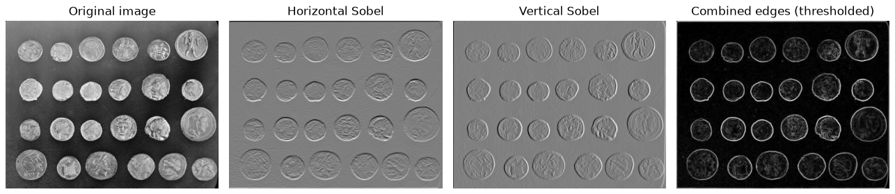
A 3×3 kernel finds edges wherever they occur. A CNN learns its kernels from data — early layers rediscover edge detectors on their own. (Sample photograph, scikit-image.)

Define convolution physically: a small set of weights (the kernel) slides across the input, computing the same weighted sum at every position. Hand-designed kernels the room may know: the mean filter blurs, Sobel filters approximate the gradient and light up edges — that is what this figure shows. The CNN’s move: stop designing kernels, learn them by gradient descent, and stack layers so later kernels combine earlier features into larger-scale patterns. The key vocabulary, stated carefully (the book’s corrected sentence): a convolution layer is translation equivariant — shift the input and the feature map shifts with it, so a pattern learned anywhere is detected everywhere. Approximate translation invariance — the same final answer wherever the pattern sits — comes from the pooling layers that discard position as they downsample. Equivariance in the features, invariance from pooling: that division of labor is the whole architecture.

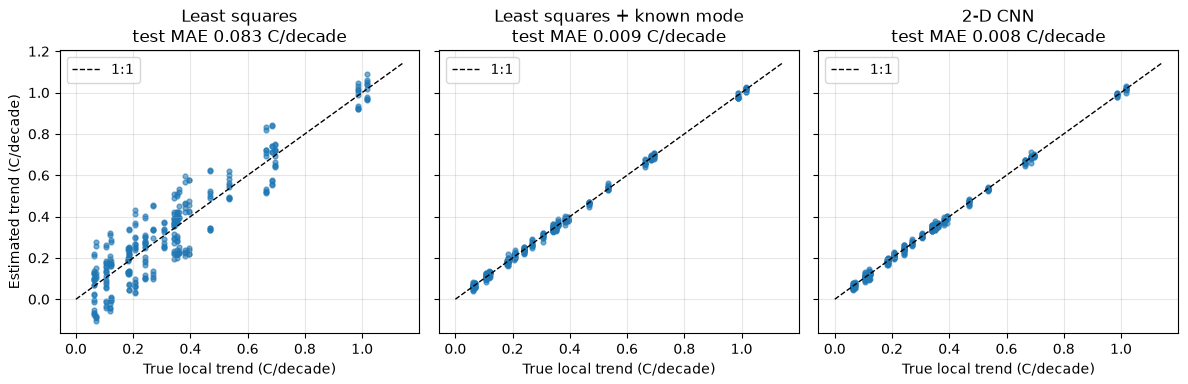
2-D case: reading a warming trend from a gridded field

The CNN beats naive least squares 10× (0.008 vs 0.083 °C/decade MAE) — but give the classical fit the one confounding mode it was missing and it matches the CNN at 0.009. A 10× win over an underspecified baseline. Synthetic (mlgeo_synth).

The task: regress each 8×8-pixel patch’s local warming trend (°C per decade) from 30 annual-mean anomaly maps stacked as channels — channels-as-time, the standard trick for time-evolving fields. Split is grouped by field (18 train, 6 test), the 3.8 doctrine applied: patches from one field never straddle the boundary. Walk the three panels left to right: naive straight-line fit, MAE 0.083 — scattered; same fit plus one extra regressor (the generator’s known 5-year interannual mode, which aliases into a straight-line slope over 30 years), MAE 0.009; the 17,953-parameter CNN, 0.008 — indistinguishable from the informed classical fit. The honest reading, say it verbatim: what the network extracted from 18 training fields is the confounding mode — deep models earn their keep when the confounders are unknown or unwritable; when you can write the physics down, the classical fit with the right regressors matches the CNN at a fraction of the cost. This is the lecture’s thesis, and the 1-D detector gets the same treatment next.

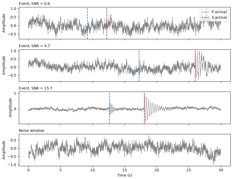
1-D case: an earthquake detector in 4,658 weights

Event windows at low SNR are invisible by eye — exactly the regime where a detector must be measured, and where real catalogs cannot measure it. Synthetic (mlgeo_synth).

The data: 1,600 30-second windows at 100 Hz from the course generator — a P arrival then a stronger S on colored noise, or noise alone — each with exact metadata: arrival times and SNR (peak signal amplitude over noise standard deviation). Point at the top trace: SNR near 0.6, nothing visible; that is where we want to know detector behavior, and real data can never tell us, because catalogs only contain the events someone already found — a bias against exactly the low-SNR regime. The model: three Conv1d–ReLU–MaxPool blocks, global average pooling, a 2-class head — 4,658 parameters against LeNet’s 61,706. Per-trace standardization first, so the network cannot classify on amplitude alone. Synthetic test accuracy: 87.9%, imperfect because the set deliberately includes near-undetectable events. The interesting question is not the average — it is where it fails. Next slide.

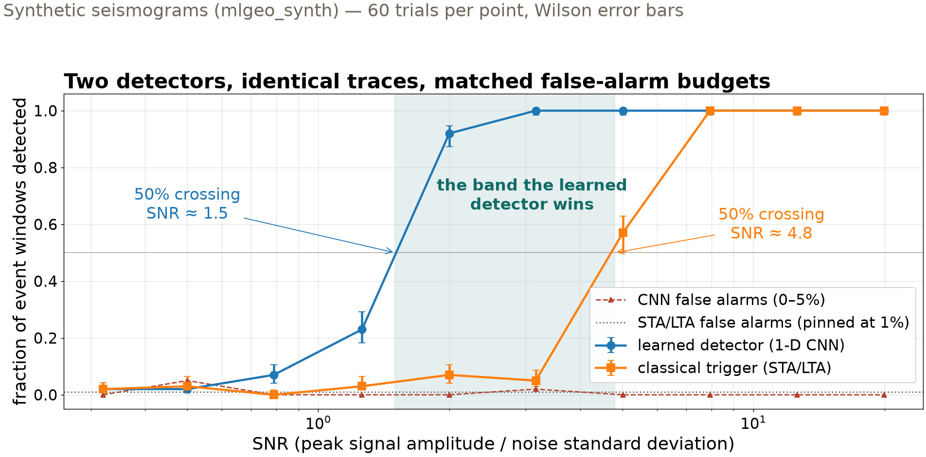
Reality check 1: same traces, classical opponent

At matched ~1% false alarms: CNN crosses 50% at SNR ≈ 1.5, the trigger at ≈ 4.8. At SNR 2 the CNN catches 92% of events; STA/LTA catches 7%. Half a decade of SNR is the entire territory the learned detector wins.

The design makes the comparison fair, and each choice is worth naming: identical traces for both detectors; the trigger’s threshold set from noise alone (99th percentile of 600 noise-only windows → 1% false alarms by construction, no peeking at events); CNN false alarms measured at 0–5%, comparable, so the detection curves can be read directly; 60 trials per point with binomial error bars. Three regimes: below SNR ~0.8 both detectors sit at their false-alarm floor — no algorithm rescues a signal buried in noise of the same color; above ~8 both detect everything, and there the classical trigger is the right engineering choice — free to train, impossible to drift. The shaded band is the CNN’s whole case. Whether that band matters is a scientific question, not an architectural one — in seismology it is where most small earthquakes live, which is why learned detectors displaced energy triggers in catalog building (Perol et al.; the pickers that followed). Also in the notebook: template matching, the classical method that beats both at low SNR when the source repeats — narrower question, different tool.

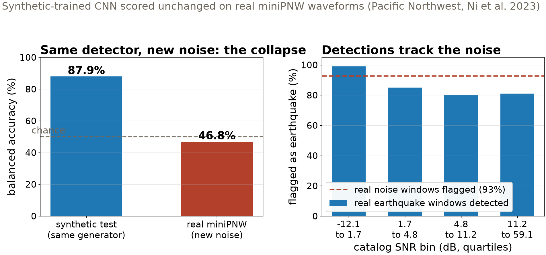
Reality check 2: real waveforms, no retraining

87.9% on synthetic test → 46.8% on real miniPNW: chance. The network flags 93% of real noise windows — it responds to Pacific Northwest microseism noise, not to earthquakes. The gap is the measurement. Real data: miniPNW (Ni et al. 2023).

The uncomfortable question the book insists on asking: every number so far came from the same generator that produced the training data — so score the unchanged detector on real labeled miniPNW waveforms (a few hundred earthquake windows, P pick 7 s in, plus matched pre-event noise windows; preprocessing mirrors training exactly, no threshold moved, no bandpass chosen to fix things afterward). Left panel: balanced accuracy collapses 41 points to chance. Right panel is the diagnosis: detection is highest (99%) in the lowest-SNR quartile — where the window is mostly noise — and the whole curve is indistinguishable from the 93% false-alarm line. The network is not responding to earthquakes at all: it learned “synthetic event vs the one synthetic noise model,” and real nonstationary, microseism-dominated noise resembles neither, so nearly everything triggers. Name the concept: distribution shift — train and deployment data drawn from different distributions — and this is Geirhos’s shortcut learning measured by us. The sentence to leave in the room: a model validated only on synthetic data has not been validated. Closing the gap takes real data on the training side (fine-tune on miniPNW, or physics-informed noise from 2.10) — that path is the notebook’s, and 4.6 continues it.

Two baselines, two verdicts

Case	Naive classical	Informed classical	CNN	Verdict
Warming trend (2-D)	0.083 °C/dec	0.009 °C/dec	0.008 °C/dec	write the physics down and they tie
Detection floor (1-D)	50% at SNR ≈ 4.8	—	50% at SNR ≈ 1.5	CNN wins the low-SNR band
Real miniPNW	—	—	46.8% (chance)	synthetic-only validation is not validation

The learned detector earns its keep only where the classical method cannot reach — and only on data from the world it was trained in.

Leave this up for questions; it is the lecture in one screen. Row 1: the CNN’s 10× headline dissolves when the classical baseline gets the one regressor it was missing — always ask what the baseline was denied. Row 2: with matched false-alarm budgets on identical traces, the CNN genuinely extends detection half a decade of SNR deeper — the honest win, and the reason this architecture took over catalog building. Row 3: the same detector, on real ground motion, is a coin flip — distribution shift eats the entire margin. The three rows are one discipline applied three times: baseline first, matched conditions, report the failure as measured. Connect forward: Monday’s forecasting shootout carries a persistence baseline row for exactly the same reason.

Now measure it yourself — open 4.3

1. pixi run jupyter lab → mlgeo_4.3_CNN.ipynb: run the convolution and LeNet warm-up quickly
2. Run the detection-floor sweep; estimate both 50% crossings from the printed table
3. Retrain with only 2 epochs, rerun the sweep: whose floor moves — the CNN’s or STA/LTA’s, and why?
4. Run the miniPNW reality check; report the balanced-accuracy gap as measured

PyTorch names live here: nn.Conv1d/nn.Conv2d, nn.MaxPool1d, nn.AdaptiveAvgPool1d, torchinfo.summary · HW-CML due today · Mon: sequence models (4.4), HW-DL assigned

Timing for the 80-minute block (10:00–11:20): pulse talks ~10 min, this deck ~20 min, guided notebook work ~40 min, synthesis ~10 min. If time is short, cut task 1 to a skim — tasks 2–4 are the payload. Task 3 is the conceptual trap worth circulating for: the CNN’s floor rises when undertrained, STA/LTA’s does not move because it has no parameters to undertrain — that is what makes it a stable baseline. Section 7 of the notebook (recoding the Rouet-Leduc tremor CNN from its published architecture table, verified by shape checks with torchinfo.summary) is the take-home skill for reading papers — flag it for project teams reproducing published models. Synthesis question to collect: for your project, what is your STA/LTA — the zero-parameter method your model must beat on identical data? That question is graded in check-in #2.