4.10 Time Series Forecast#

1. Introduction: The Importance of Time Series Forecasting in Geoscientific Research#

Time series forecasting has been a cornerstone of geoscientific research, providing essential insights into Earth system processes and enabling proactive decision-making in diverse applications. From predicting seasonal climate patterns and river discharge to monitoring seismic activity and volcanic eruptions, time series analysis offers a powerful framework to understand temporal trends, cycles, and anomalies in geophysical data.

Why Time Series Forecasting Matters in Geosciences

Climate and Weather Forecasting:
Seasonal and interannual climate variations, such as the El Niño-Southern Oscillation (ENSO), have profound impacts on agriculture, water resources, and disaster preparedness. Accurate forecasting helps manage risks associated with droughts, floods, and heatwaves.
Hydrology and Water Resource Management:
Streamflow and reservoir inflow forecasting are critical for managing water supplies, especially in regions prone to water scarcity or flooding.
Seismic and Volcanic Monitoring:
While precise prediction of earthquakes remains elusive, forecasting the likelihood of seismic events based on past activity patterns can guide hazard mitigation strategies. Similarly, time series data from volcanic monitoring systems provide early warning for eruptions.
Oceanography and Marine Ecosystems:
Forecasting changes in sea surface temperatures and ocean currents informs fisheries management and helps monitor phenomena like coral bleaching and ocean acidification.
Renewable Energy:
Forecasting solar radiation and wind patterns enables efficient integration of renewable energy sources into power grids.

Revival of Interest with AI and Deep Learning In recent years, the advent of AI and deep learning models such as recurrent neural networks (RNNs), transformers, and even large language models (LLMs) has revolutionized time series forecasting. These models:

Capture complex temporal dependencies and nonlinear patterns in ways that traditional statistical models often cannot.
Enable integration of diverse geoscientific datasets, including time series with spatial and multivariate dimensions.
Open new frontiers in tackling previously intractable problems, such as long-term climate forecasting and predicting rare geophysical events.

Goals of the Lecture In this lecture, we will:

Explore the role of time series forecasting in geoscientific research.
Develop and analyze a geoscientifically inspired toy dataset.
Compare approaches:
- Baseline statistical models for their simplicity and robustness.
- Classic machine learning models to understand feature engineering and generalization.
- Deep learning models to harness the power of neural networks for temporal prediction.
Evaluate these methods in terms of their predictive performance, interpretability, and scalability to real-world geoscientific problems.

2. Important Concepts in Time series forecasting#

Context In statistical learning, the context in a time series can refer to the historical data or the portion of the past observations used to predict future values. This historical context is essential for capturing temporal dependencies, trends, seasonality, and other repeating patterns. The amount of context needed depends on the nature of the dataset—for instance, long-term climatic forecasts often require years of past data, while seismic activity predictions may focus on shorter, event-driven contexts. In scientific inquiry, the context might be the scientific knowledge or additional “covariate” (e.g., temperature and precipitation) that might help inform the forecast.
Look-Back Window defines the specific number of past time steps used as input to the forecasting model, equivalent to the context. For example:
- A short look-back window might capture local or short-term dependencies (e.g., hourly temperature changes).
- A long look-back window can capture more extended trends and seasonal patterns (e.g., annual temperature cycles). Choosing an appropriate look-back window is a balance: too short and the model may miss important patterns, too long and it may include irrelevant or noisy data.
Horizon refers to how far into the future the model predicts. This can range from:
- Short-term horizons, such as the next hour or day, where temporal dependencies are strong and relatively predictable.
- Long-term horizons, such as monthly or annual predictions, where uncertainty grows due to external influences, stochastic variability, and system non-linearity.
- Prediction Length defines the number of future time steps forecasted in a single prediction. Models can be designed to:
Increasing Uncertainty with Longer Horizons Forecast accuracy generally decreases as the prediction horizon lengthens. This is because:
- Error propagation: In multi-step predictions, small errors in early predictions compound as they are fed into the model for subsequent predictions.
- Complexity of future influences: Longer horizons are more affected by external and often unpredictable factors, such as sudden climatic events or anomalous geophysical activity.
- Loss of signal strength: Temporal correlations weaken over time, making it harder for models to extract meaningful patterns for far-future predictions.

3. Toy Dataset#

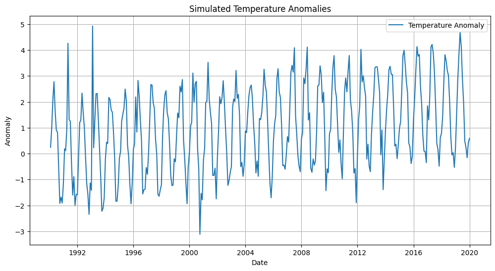
We’ll generate synthetic geoscientific time series data simulating monthly surface temperature anomalies for a fictional region over 30 years. The data will incorporate:

Seasonality: A sinusoidal signal with annual cycles.
Trend: A small upward trend over time (e.g., global warming).
Noise: Gaussian noise to simulate variability.
Anomalies: Sudden deviations simulating geoscientific events like volcanic eruptions or ENSO effects.

import numpy as np
import pandas as pd

# Generate time series
np.random.seed(42)
time = pd.date_range(start='1990-01-01', end='2019-12-31', freq='M')
n = len(time)

# Components
trend = np.linspace(0, 2, n)  # Linear trend
seasonality = 2 * np.sin(2 * np.pi * (np.arange(n) % 12) / 12)  # Annual cycle
noise = np.random.normal(0, 0.5, n)  # Random noise
anomalies = np.zeros(n)
anomalies[np.random.choice(n, 5, replace=False)] = np.random.uniform(-5, 5, 5)  # Sudden anomalies

# Final series
temperature_anomalies = trend + seasonality + noise + anomalies

# Create DataFrame
data = pd.DataFrame({'Date': time, 'Temperature_Anomaly': temperature_anomalies})
data.set_index('Date', inplace=True)
data.to_csv('geoscientific_time_series.csv')
data.head()

	Temperature_Anomaly
Date
1990-01-31	0.248357
1990-02-28	0.936439
1990-03-31	2.067037
1990-04-30	2.778228
1990-05-31	1.637258

# plot the data
import matplotlib.pyplot as plt
plt.figure(figsize=(12, 6))
plt.plot(data.index, data['Temperature_Anomaly'], label='Temperature Anomaly')
plt.title('Simulated Temperature Anomalies')
plt.xlabel('Date')
plt.ylabel('Anomaly')
plt.grid()
plt.legend()
plt.show()

../_images/mlgeo_4.10_timeseriesforecast_2_0.png

Define Context and Horizon

Given this long time series, we will focus on making a rolling forecast by defining a context and a horizon window.

# define a context and a horizon window
context_window = 12
horizon_window = 6

# Split data into train/test, which is basically the context (train) and horizon (test)
train = data['Temperature_Anomaly'][:-horizon_window] # context window here is the entire thing
test = data['Temperature_Anomaly'][-horizon_window:]

3. Forecasting Methods#

3.1 Baseline: Statistical Forecasts#

Naive Forecast: Use the last observed value as the next prediction.
Seasonal Naive Forecast: Use the value from the same season in the previous year.
ARIMA: Fit an AutoRegressive Integrated Moving Average model.

from statsmodels.tsa.arima.model import ARIMA
from sklearn.metrics import mean_squared_error

# Naive Forecast
naive_forecast = np.array([train.iloc[-1]] * horizon_window)
naive_rmse = np.sqrt(mean_squared_error(test, naive_forecast))
naive_mae = np.mean(np.abs(test - naive_forecast))

# seasonal naive forecast
seasonal_naive_forecast = np.array([train.iloc[-12]] * horizon_window)
seasonal_naive_rmse = np.sqrt(mean_squared_error(test, seasonal_naive_forecast))
seasonal_naive_mae = np.mean(np.abs(test - seasonal_naive_forecast))

# ARIMA Model
arima_model = ARIMA(train, order=(2, 1, 2)).fit()
arima_forecast = arima_model.forecast(steps=horizon_window)
arima_rmse = np.sqrt(mean_squared_error(test, arima_forecast))
arima_mae = np.mean(np.abs(test - arima_forecast))

# report all evaluation metrics
print(f"Naive RMSE: {naive_rmse}, Naive MAE: {naive_mae}")
print(f"Seasonal Naive RMSE: {seasonal_naive_rmse}, Seasonal Naive MAE: {seasonal_naive_mae}")
print(f"ARIMA RMSE: {arima_rmse}, ARIMA MAE: {arima_mae}")

/Users/marinedenolle/opt/miniconda3/envs/mlgeo/lib/python3.9/site-packages/statsmodels/tsa/base/tsa_model.py:473: ValueWarning: No frequency information was provided, so inferred frequency M will be used.
  self._init_dates(dates, freq)
/Users/marinedenolle/opt/miniconda3/envs/mlgeo/lib/python3.9/site-packages/statsmodels/tsa/base/tsa_model.py:473: ValueWarning: No frequency information was provided, so inferred frequency M will be used.
  self._init_dates(dates, freq)
/Users/marinedenolle/opt/miniconda3/envs/mlgeo/lib/python3.9/site-packages/statsmodels/tsa/base/tsa_model.py:473: ValueWarning: No frequency information was provided, so inferred frequency M will be used.
  self._init_dates(dates, freq)

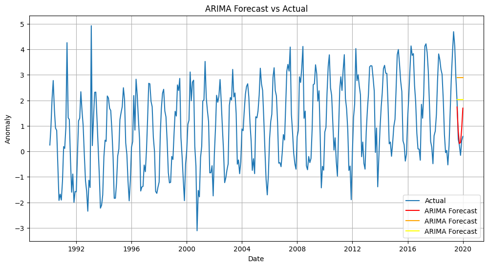
Naive RMSE: 2.389823903102479, Naive MAE: 2.2973182078545107
Seasonal Naive RMSE: 1.5820363949721554, Seasonal Naive MAE: 1.4384894213432322
ARIMA RMSE: 0.5550037051446414, ARIMA MAE: 0.4465414221142508

/Users/marinedenolle/opt/miniconda3/envs/mlgeo/lib/python3.9/site-packages/statsmodels/base/model.py:607: ConvergenceWarning: Maximum Likelihood optimization failed to converge. Check mle_retvals
  warnings.warn("Maximum Likelihood optimization failed to "

# plot the three predictions from the base models
plt.figure(figsize=(12, 6))
plt.plot(data.index, data['Temperature_Anomaly'], label='Actual')
plt.plot(test.index, arima_forecast, label='ARIMA Forecast', color='red')
plt.plot(test.index, naive_forecast, label='ARIMA Forecast', color='orange')
plt.plot(test.index, seasonal_naive_forecast, label='ARIMA Forecast', color='yellow')
plt.title('ARIMA Forecast vs Actual')
plt.xlabel('Date')
plt.ylabel('Anomaly')
plt.grid()
plt.legend()
plt.show()

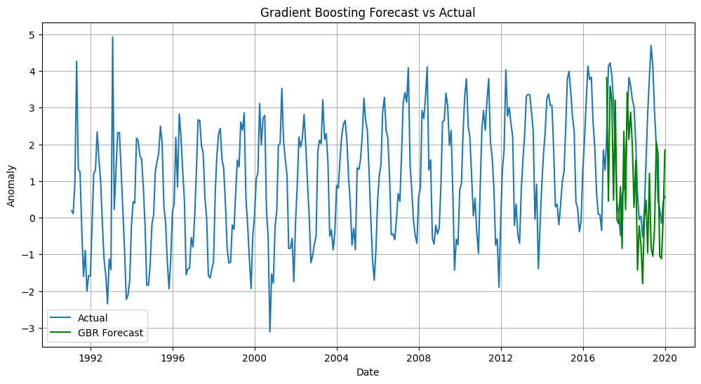
../_images/mlgeo_4.10_timeseriesforecast_8_0.png

3.2. Classic Machine Learning#

Use Lag Features and Seasonality Features as input.
Algorithms: Linear Regression, Random Forest, Gradient Boosting.

from sklearn.ensemble import GradientBoostingRegressor
from sklearn.model_selection import train_test_split

# Create context features
for lag in range(1, context_window + 1):
    data[f'Lag_{lag}'] = data['Temperature_Anomaly'].shift(lag) # shift the data
data.dropna(inplace=True)


# Create training data as the past, test data as the future 
X = data.iloc[:, 1:].values
y = data['Temperature_Anomaly'].values

X_train, X_test, y_train, y_test = train_test_split(X, y, test_size=0.1, random_state=42)

# Gradient Boosting Regressor
model = GradientBoostingRegressor()
model.fit(X_train, y_train)
y_pred = model.predict(X_test)

# Evaluate
gbr_rmse = np.sqrt(mean_squared_error(y_test, y_pred))
gbr_mae = np.mean(np.abs(y_test - y_pred))
print(f"Gradient Boosting RMSE: {gbr_rmse} , Gradient Boosting MAE: {gbr_mae}")

# plot the predictions
plt.figure(figsize=(12, 6))
plt.plot(data.index, data['Temperature_Anomaly'], label='Actual')
plt.plot(data.index[-len(y_test):], y_pred, label='GBR Forecast', color='green')
plt.title('Gradient Boosting Forecast vs Actual')
plt.xlabel('Date')
plt.ylabel('Anomaly')
plt.grid()
plt.legend()

Gradient Boosting RMSE: 0.6784327786162885 , Gradient Boosting MAE: 0.5225129530636484

<matplotlib.legend.Legend at 0x30ca181c0>

../_images/mlgeo_4.10_timeseriesforecast_10_2.png

3.3 Deep Learning#

Models: RNNs, LSTMs, GRUs, or Transformers.
Framework: PyTorch.

import torch
import torch.nn as nn
from torch.utils.data import DataLoader, Dataset

# Custom dataset for PyTorch
class TimeSeriesDataset(Dataset):
    def __init__(self, data, context_window, horizon_window):
        self.X = [data[i:i + context_window] for i in range(len(data) - (context_window+horizon_window))]
        self.y = [data[i+context_window:i+context_window+horizon_window] for i in range(len(data) - (context_window+horizon_window))]
    
    def __len__(self):
        return len(self.y)
    
    def __getitem__(self, idx):
        return torch.tensor(self.X[idx], dtype=torch.float32), torch.tensor(self.y[idx], dtype=torch.float32)

# RNN Model
class RNNModel(nn.Module):
    def __init__(self, input_size, hidden_size, num_layers, output_size):
        super(RNNModel, self).__init__()
        self.rnn = nn.RNN(input_size, hidden_size, num_layers, batch_first=True)
        self.fc = nn.Linear(hidden_size, output_size)
    
    def forward(self, x):
        _, h_n = self.rnn(x)
        out = self.fc(h_n[-1])
        return out

# Prepare data
ts_data = TimeSeriesDataset(data['Temperature_Anomaly'].values, context_window, horizon_window)
dataloader = DataLoader(ts_data, batch_size=16, shuffle=True)

# Model, loss, and optimizer
print(context_window, horizon_window)
model = RNNModel(input_size=context_window, hidden_size=50, num_layers=4, output_size=horizon_window)
criterion = nn.MSELoss()
optimizer = torch.optim.Adam(model.parameters(), lr=0.001)

12 6

# Training loop
for epoch in range(50):
    epoch_loss = 0
    for X_batch, y_batch in dataloader:
        # X_batch = X_batch.unsqueeze(-1)  # Add feature dimension
        y_pred = model(X_batch).squeeze()
        loss = criterion(y_pred, y_batch)
        optimizer.zero_grad()
        loss.backward()
        optimizer.step()
        epoch_loss += loss.item()
    print(f'Epoch: {epoch}, Loss: {epoch_loss/len(dataloader)}')

Epoch: 0, Loss: 3.00634267216637
Epoch: 1, Loss: 2.6486164728800454
Epoch: 2, Loss: 2.626796557789757
Epoch: 3, Loss: 2.6268500714074996
Epoch: 4, Loss: 2.6511067549387612
Epoch: 5, Loss: 2.6555847894577753
Epoch: 6, Loss: 2.6372431346348355
Epoch: 7, Loss: 2.627526181084769
Epoch: 8, Loss: 2.7000722998664495
Epoch: 9, Loss: 2.6251020034154258
Epoch: 10, Loss: 2.608908255894979
Epoch: 11, Loss: 2.613211399032956
Epoch: 12, Loss: 2.6141854581378756
Epoch: 13, Loss: 2.620620619683039
Epoch: 14, Loss: 2.624014150528681
Epoch: 15, Loss: 2.605562698273432
Epoch: 16, Loss: 2.6024255752563477
Epoch: 17, Loss: 2.585343973977225
Epoch: 18, Loss: 2.5852765242258706
Epoch: 19, Loss: 2.665037166504633
Epoch: 20, Loss: 2.6180632625307356
Epoch: 21, Loss: 2.6397100516727994
Epoch: 22, Loss: 2.572316567103068
Epoch: 23, Loss: 2.571771576291039
Epoch: 24, Loss: 2.616808993475778
Epoch: 25, Loss: 2.5992123512994674
Epoch: 26, Loss: 2.5893679005759105
Epoch: 27, Loss: 2.5868957894189015
Epoch: 28, Loss: 2.5527749913079396
Epoch: 29, Loss: 2.5988870348249162
Epoch: 30, Loss: 2.5735259453455606
Epoch: 31, Loss: 2.615531495639256
Epoch: 32, Loss: 2.623429911477225
Epoch: 33, Loss: 2.567932753335862
Epoch: 34, Loss: 2.588108857472738
Epoch: 35, Loss: 2.569101481210618
Epoch: 36, Loss: 2.5912431478500366
Epoch: 37, Loss: 2.5857595716203963
Epoch: 38, Loss: 2.5676723207746233
Epoch: 39, Loss: 2.5795442263285318
Epoch: 40, Loss: 2.622153815769014
Epoch: 41, Loss: 2.598675188564119
Epoch: 42, Loss: 2.568843750726609
Epoch: 43, Loss: 2.5866817860376266
Epoch: 44, Loss: 2.631495998019264
Epoch: 45, Loss: 2.6336796397254583
Epoch: 46, Loss: 2.586955535979498
Epoch: 47, Loss: 2.6301064434505643
Epoch: 48, Loss: 2.585471754982358
Epoch: 49, Loss: 2.547369820731027

# Evaluate
test_input = torch.tensor(data['Temperature_Anomaly'].values[-(context_window+horizon_window):-horizon_window].reshape(1,-1), dtype=torch.float32)
rnn_forecast = model(test_input).detach().numpy()

from sklearn.metrics import mean_squared_error, mean_absolute_error

# Assuming test contains the ground truth values for the last 12 months
ground_truth = data['Temperature_Anomaly'][-horizon_window:].values

# Calculate RMSE
rnn_rmse = np.sqrt(mean_squared_error(ground_truth, rnn_forecast))
print(f"RNN RMSE: {rnn_rmse}")

# Calculate MAE
rnn_mae = mean_absolute_error(ground_truth, rnn_forecast)
print(f"RNN MAE: {rnn_mae}")

RNN RMSE: 0.64634883661374
RNN MAE: 0.47775794587681136

4. Comparison and Discussion#

Evaluation Metrics:
1. Mean Squared Error (MSE)
  - Use: Measures the average squared difference between predicted and actual values. It penalizes larger errors more heavily.
  - Considerations: While useful, MSE doesn’t account for trends or seasonal components, making it potentially less informative for complex time series (e.g., those with strong seasonality).
  - Best for: General forecasts when trends and magnitudes of errors are important.
2. Mean Absolute Error (MAE)
  - Use: Measures the average of the absolute errors. Unlike MSE, it doesn’t heavily penalize outliers.
  - Considerations: MAE can be more robust when there are outliers, which is common in power-law distributed data. However, it also doesn’t account for trends or periodicity.
  - Best for: Situations where the model needs to be evaluated without over-penalizing large errors (e.g., for power-law distributions).
3. Root Mean Squared Error (RMSE)
  - Use: RMSE is the square root of MSE, offering a more interpretable metric in terms of the units of the original data.
  - Considerations: Like MSE, it is sensitive to outliers. For time series with strong trends, RMSE can be large if forecasts consistently lag or lead trends.
  - Best for: General forecasting, but less ideal for highly seasonal or trending data unless seasonality is detrended.
4. Mean Absolute Percentage Error (MAPE)
  - Use: Measures the percentage error between the forecast and the actual value. It normalizes the error by the magnitude of the actual values.
  - Considerations: MAPE can be problematic when actual values are close to zero (leading to high percentages). It is also less effective for power-law distributions where low-frequency, high-magnitude events can skew the results.
  - Best for: Forecasts where relative error matters more than absolute error, especially for non-power-law distributed data.
5. Symmetric Mean Absolute Percentage Error (sMAPE)
  - Use: A variation of MAPE that adjusts for issues with division by zero and symmetry in errors.
  - Considerations: Like MAPE, it works better for data without extreme outliers or heavy-tailed distributions.
  - Best for: Relative error measurement, especially for periodic or seasonal data where symmetry in error matters.
6. Mean Squared Logarithmic Error (MSLE)
  - Use: Useful when the forecast error should be penalized more when underestimating than when overestimating, especially for datasets with a wide dynamic range.
  - Considerations: Works well for power-law distributions or data with large variations in scale, as it compresses the impact of large errors.
  - Best for: Power-law distributed data where large-magnitude events need reduced influence.
7. Autocorrelation of Residuals
  - Use: Measures whether forecast errors (residuals) are correlated over time, indicating if the model has captured the structure of the data.
  - Considerations: Important for time series with periodicity, as autocorrelated residuals suggest that the model has failed to account for recurring patterns or cycles.
  - Best for: Time series with strong periodicity or seasonality.
8. Trend-Corrected Metrics:
  - Use: Metrics like Mean Absolute Scaled Error (MASE) help correct for trend or seasonality. MASE normalizes the error by a benchmark model (e.g., a naïve forecast).
  - Considerations: It adjusts for trend and seasonality, making it more reliable for data that has both components.
  - Best for: Data with both trends and periodicity.
9. Spectral Score (for Periodic Data)
  - Use: Measures the alignment between the frequency components of the forecast and the actual data, useful for evaluating models on data with clear periodicity.
  - Considerations: This metric focuses on the frequency domain, complementing time-domain error metrics for highly periodic or cyclical data.
  - Best for: Time series dominated by periodicity or cyclical patterns.
10. Quantile Loss/Pinball Loss
- Use: Evaluates the forecast’s ability to predict different quantiles, especially useful when forecasting intervals or uncertainty bounds.
- Considerations: Works well with power-law distributions where you care about upper or lower tail behavior (e.g., rare but extreme events).
- Best for: Time series with significant outliers or fat-tailed distributions.
1. Directional Accuracy
- Use: Measures whether the forecast correctly predicts the direction of change (up or down).
- Considerations: In trending time series, this metric helps assess whether the forecast captures the general movement.
- Best for: Data with strong trends, where capturing the direction of change is more important than minimizing the magnitude of error.

Metric Selection Based on Data Characteristics

Trends: Use trend-corrected metrics (MASE) and directional accuracy. Combine with RMSE or MAE to evaluate overall fit.
Periodicity: Autocorrelation of residuals, spectral score, or sMAPE.
Power-Law Distributions: Quantile loss, MSLE, or robust metrics like MAE that handle outliers better than squared-error metrics.

import pandas as pd
import numpy as np

# Assuming you have the RMSE and MAE values for each model
# Replace these values with the actual values from your models
results = {
    'Model': ['Baseline', 'CML', 'DL'],
    'RMSE': [arima_rmse, gbr_rmse, rnn_mae],  # Replace with actual RMSE values
    'MAE': [arima_rmse, gbr_rmse, rnn_rmse]    # Replace with actual MAE values
}

# Create a DataFrame to store the results
results_df = pd.DataFrame(results)

# Print the results table
print(results_df)

# Save the results to a CSV file
results_df.to_csv('model_performance_comparison.csv', index=False)

      Model      RMSE       MAE
Baseline  0.555004  0.555004
     CML  0.678433  0.678433
      DL  0.477758  0.646349

5. Testing Foundation Models#

In this example, we will test Chronos on canonical geoscientific data sets chosen to be representative of geoscience/geophysics:

earthquake catalogs from SoCal
earthquake ground motion waveforms
near surface properties (seismic velocities, temperature, soil moisture)
ice velocity from greenland
GPS positions along a plate boundary that captures seasons and tectonic loading. The data files are gathered on this repository: https://github.com/UW-MLGEO/MLGeo-dataset

The data has been prepared as CSV files with times series. The forescasts are added to the CSV files under key attributes “Chronos-zero-shot”.

Limitations by Chronos. Chronos uses large language models at its core for forecasting time series. The time series is “tokenized” to convert from an array of floats into contect tokens.

By Marine Denolle (mdenolle@uw.edu)

! pip install chronos-forecasting

import torch
torch.cuda.empty_cache()
import gc
gc.collect()

import matplotlib.pyplot as plt
import torch
from chronos import ChronosPipeline, ChronosBoltPipeline
import pandas as pd
import numpy as np


# Set the font style and size
plt.rcParams.update({
    'font.size': 12,
    'font.family': 'sans-serif',
    'font.serif': ['DejaVu Sans'],
    'axes.titlesize': 12,
    'axes.labelsize': 10,
    'xtick.labelsize': 10,
    'ytick.labelsize': 10,
    'legend.fontsize': 10
})

# benchmarking with ARIMA
!pip install statsmodels
from statsmodels.tsa.arima.model import ARIMA

# Assuming df is your DataFrame and 'datetime' is your datetime column
# df["datetime"] = pd.to_datetime(df["datetime"])
# df.set_index("datetime", inplace=True)

# # Assuming 'value' is the column you want to forecast
# data = df['value']

# Fit ARIMA model
# model = ARIMA(data, order=(5, 1, 0))  # (p, d, q) order, adjust as needed
# model_fit = model.fit()

# # Make predictions
# forecast_steps = 10  # Number of steps to forecast
# forecast = model_fit.forecast(steps=forecast_steps)

# # Plot the results
# plt.figure(figsize=(10, 6))
# plt.plot(data, label='Actual')
# plt.plot(forecast, label='Forecast', color='red')
# plt.legend()
# plt.show()

# # Print forecasted values
# print(forecast)

n_timeseries = 20

pipeline = ChronosBoltPipeline.from_pretrained(
    "amazon/chronos-bolt-base",
    device_map="cuda",  # use "cpu" for CPU inference and "mps" for Apple Silicon
    torch_dtype=torch.bfloat16,
)

from chronos import BaseChronosPipeline, ChronosPipeline, ChronosBoltPipeline

print(BaseChronosPipeline.predict.__doc__)  # for Chronos models
print(ChronosPipeline.predict.__doc__)  # for Chronos models

        Get forecasts for the given time series. Predictions will be
        returned in fp32 on the cpu.

        Parameters
        ----------
        context
            Input series. This is either a 1D tensor, or a list
            of 1D tensors, or a 2D tensor whose first dimension
            is batch. In the latter case, use left-padding with
            ``torch.nan`` to align series of different lengths.
        prediction_length
            Time steps to predict. Defaults to a model-dependent
            value if not given.

        Returns
        -------
        forecasts
            Tensor containing forecasts. The layout and meaning
            of the forecasts values depends on ``self.forecast_type``.
        

        Get forecasts for the given time series.

        Refer to the base method (``BaseChronosPipeline.predict``)
        for details on shared parameters.

        Additional parameters
        ---------------------
        num_samples
            Number of sample paths to predict. Defaults to what
            specified in ``self.model.config``.
        temperature
            Temperature to use for generating sample tokens.
            Defaults to what specified in ``self.model.config``.
        top_k
            Top-k parameter to use for generating sample tokens.
            Defaults to what specified in ``self.model.config``.
        top_p
            Top-p parameter to use for generating sample tokens.
            Defaults to what specified in ``self.model.config``.
        limit_prediction_length
            Force prediction length smaller or equal than the
            built-in prediction length from the model. False by
            default. When true, fail loudly if longer predictions
            are requested, otherwise longer predictions are allowed.

        Returns
        -------
        samples
            Tensor of sample forecasts, of shape
            (batch_size, num_samples, prediction_length).
        

print(ChronosBoltPipeline.predict.__doc__)  # for Chronos-Bolt models

        Get forecasts for the given time series.

        Refer to the base method (``BaseChronosPipeline.predict``)
        for details on shared parameters.
        Additional parameters
        ---------------------
        limit_prediction_length
            Force prediction length smaller or equal than the
            built-in prediction length from the model. False by
            default. When true, fail loudly if longer predictions
            are requested, otherwise longer predictions are allowed.

        Returns
        -------
        torch.Tensor
            Forecasts of shape (batch_size, num_quantiles, prediction_length)
            where num_quantiles is the number of quantiles the model has been
            trained to output. For official Chronos-Bolt models, the value of
            num_quantiles is 9 for [0.1, 0.2, ..., 0.9]-quantiles.

        Raises
        ------
        ValueError
            When limit_prediction_length is True and the prediction_length is
            greater than model's trainig prediction_length.
        

Some functions

def reshape_time_series(df, name_of_target="count" ,n_timeseries=20, duration_years=2):
    """
    Generate a list of time series from the given DataFrame.

    Parameters:
    df (pd.DataFrame): The input DataFrame containing a 'datetime' column.
    n_timeseries (int): Number of time series to generate.
    duration_years (int): Duration of each time series in years.
    resample_period (str): Resampling period (e.g., 'D' for daily).

    Returns:
    list: A list of DataFrames, each containing a time series.
    pd.DataFrame: A wide-format DataFrame containing the time series.
    """
    df_list = [pd.DataFrame() for _ in range(n_timeseries)]
    kk = 0
    while kk < n_timeseries:
        start_date = df["datetime"].sample().values[0]
        start_date = pd.to_datetime(start_date)
        # Create a time series for the specified duration
        end_date = start_date + pd.DateOffset(years=duration_years)
        if end_date > df["datetime"].max():
            continue    # Skip if the end date exceeds the maximum date in the catalog
        # Create a time series from the catalog and select only the date time and target columns
        time_series = df[(df["datetime"] >= start_date) & (df["datetime"] <= end_date)][["datetime", name_of_target]]
        time_series = time_series.set_index("datetime")
        # time_series = time_series.resample(resample_period).mean().interpolate() # resample and interpolate
        time_series = time_series.ffill()#(method="ffill") # forward fill
        time_series = time_series.bfill()#(method="bfill") # backward fill
        time_series = time_series.reset_index()# reset index to keep datetime as a column
        # remove the "datetime" column to the time_series
        
        df_list[kk] = time_series
        kk += 1 
    df_list_count = [pd.DataFrame() for _ in range(n_timeseries)]
    for ik in range(n_timeseries):
        df_list_count[ik] = df_list[ik][name_of_target]
        df_list_count[ik] = df_list_count[ik].rename(f"target_{ik}")
    df_wide = pd.concat(df_list_count, axis=1)

    # find the sampling rate dt as the difference between the first two dates
    dt = df["datetime"].diff().dt.total_seconds().fillna(0).mean()
    # convert dt to days
    dt = dt / (24 * 3600)
    print("sampling rate {:.2f} days".format(dt))

    # create a time array that is the index of the time series and convert the dae
    df_wide["time_index"] = np.arange(len(df_wide)) #* pd.Timedelta(days=dt)
    # move the last column to the first position
    cols = df_wide.columns.tolist()
    cols = cols[-1:] + cols[:-1]
    df_wide = df_wide[cols]

    # rename columns to target_ID except for the first column that is a datetime
    df_wide.columns = [f"target_{i}" if i != 0 else "time_index" for i in range(len(df_wide.columns))]
    df_wide = df_wide.dropna() 
    
    return df_list, df_wide

# Example usage:
# df_list,df_wide = reshape_time_series(df, n_timeseries=20, duration_years=2, resample_period='D')

def predict_chronos(df, predict_length=64, n_timeseries=20):
    """
    Make predictions for the given time series data.

    Parameters:
    df (pd.DataFrame): The input DataFrame containing the time series data.

    Returns:
    forecast_mean (np.array): The mean forecasted values for the time series.
    lower_bound (np.array): The 5% lower bound of the forecasted values.
    upper_bound (np.array): The 95% upper bound of the forecasted values.
    mean_mae (float): The mean absolute error of the forecasted values.
    no_var_mae (float): The mean absolute error assuming no change in the time series.


    """
    # Ensure df['Date'] is in datetime format
    # df['datetime'] = pd.to_datetime(df['datetime'])

    # Select the first n_timeseries columns for forecasting
    columns_to_forecast = df.columns[1:n_timeseries+1]  # +1 to skip the 'Date' column

    # Calculate the split index for training
    split_index = int(len(df) - predict_length)

    # Split the data into training and evaluation sets for all selected columns
    train_data = df[columns_to_forecast].iloc[:split_index]
    eval_data = df[columns_to_forecast].iloc[split_index:]

    # Convert the training data to a higher-dimensional tensor
    train_tensor = torch.tensor(train_data.values, dtype=torch.float32).T
    # Perform the forecasting using the training data
    # forecast = pipeline.predict(
    #     context=train_tensor,
    #     prediction_length=len(eval_data),  # Predict the same length as the evaluation set
    #     num_samples=50,
    # )
    forecast = pipeline.predict(
        context=train_tensor,
        prediction_length=len(eval_data))  # Predict the same length as the evaluation set
    # )

    # Take the mean across the samples (axis=1) for each time series
    forecast_mean = forecast.mean(dim=1).squeeze().numpy()
    # lower_bound = forecast.quantile(0.05, dim=1).squeeze().numpy()
    # upper_bound = forecast.quantile(0.95, dim=1).squeeze().numpy()


    mae=[]
    # Calculate and print the MAE for each time series
    for i, column_name in enumerate(columns_to_forecast):
        # Calculate MAE for the current time series
        mae.append (np.mean(np.abs(forecast_mean[i]- eval_data[column_name].values)))
        
        # Print the MAE
        print(f'Mean Absolute Error (MAE) for {column_name}: {mae[-1]}')

    mean_mae = np.array(mae).mean()
    print(f'Mean of forecast MAEs = {mean_mae}')

    # Calculate and print the MASE for each time series
    mase=[]
    for i, column_name in enumerate(columns_to_forecast):
        # Calculate MASE for the current time series
        mase.append (np.mean(np.abs(forecast_mean[i] - eval_data[column_name].values)) / np.mean(np.abs(eval_data[column_name].values[1:] - eval_data[column_name].values[:-1])))
        
        # Print the MASE
        print(f'Mean Absolute Scaled Error (MASE) for {column_name}: {mase[-1]}')

    mean_mase = np.array(mase).mean()
    print(f'Mean of forecast MAEs = {mean_mase}')


    # Baseline model: ARIMA
    mae_arima=[]
    # Calculate and print the MAE for each time series
    for i, column_name in enumerate(columns_to_forecast):
        # Calculate MAE for the current time series
        mae_arima.append (np.mean(np.abs(eval_data[column_name].values[-1] - eval_data[column_name].values)))
        
        # Print the MAE
        # print(f'MAE assuming d/dt=0 for {column_name}: {mae_nochangemodel[-1]}')

    mae_arima_mean = np.array(mae_arima).mean()
    print(f'Mean of ARIMA MAEs = {mae_arima_mean}')

    return forecast,mean_mae, mean_mase, mae_arima_mean, split_index

import matplotlib.dates as mdates
def plot_forecasts(df_wide,split_index,forecast,n_timeseries,field="count",filename="geo-forecast.png"):
    """
    Plot the forecasted values along with the confidence intervals.

    Parameters:
    n_timeseries (int): Number of time series to plot.
    df_wide (pd.DataFrame): The wide-format DataFrame containing the time series.
    split_index (int): The index at which the training data ends (or context data) and evaluation (or forecast) data begins.
    forecast (np.array): The forecasted values for the time series.
    filename (str): The filename to save the plot.


    Returns:
    None


    """
    
    # Determine the number of rows and columns for the subplots
    n_timeseries = min(n_timeseries, 12)  # Cap the number of time series to 12
    nrows = (n_timeseries - 1) // 3 + 1
    ncols = min(n_timeseries, 3)

    # Select the first n_timeseries columns for forecasting
    columns_to_forecast = df_wide.columns[1:n_timeseries+1]  # +1 to skip the 'Date' column
    print(forecast.shape)
    forecast_mean = forecast.mean(dim=1).squeeze()
    print(forecast_mean.shape)
    lower_bound = np.percentile(forecast, 5, axis=0)
    upper_bound = np.percentile(forecast, 95, axis=0)

    # Layout the subplots
    fig, axes = plt.subplots(nrows, ncols, figsize=(20, 16), sharex=True)
    # Flatten the 2D array of axes for easy indexing
    if n_timeseries>1:
        axes = axes.flatten()
    else:
        axes = [axes]
        


    # Split the data into training and evaluation sets for all selected columns
    # train_data = df_wide[columns_to_forecast].iloc[:split_index]
    eval_data = df_wide[columns_to_forecast].iloc[split_index:]


    # Calculate and print the MASE for each time series
    mase=[]
    for i, column_name in enumerate(columns_to_forecast):
        # Calculate MASE for the current time series
        mase.append (np.mean(np.abs(forecast_mean[i].numpy()  - eval_data[column_name].values)) / np.mean(np.abs(eval_data[column_name].values[1:] - eval_data[column_name].values[:-1])))
        
    mean_mase = np.array(mase).mean()
    print(f'Mean of forecast MASEs = {mean_mase}')
    print(n_timeseries)
    # Iterate over the first n_timeseries and plot
    if n_timeseries>1:
        for i, column_name in enumerate(columns_to_forecast[0:n_timeseries]):
            # Plot the original data
            axes[i].plot(df_wide['time_index'], df_wide[column_name], label='Original Data')
            
            # Calculate the 5th and 95th percentiles for the confidence interval
            lower_bound = np.percentile(forecast[i, :, :], 5, axis=0)
            upper_bound = np.percentile(forecast[i, :, :], 95, axis=0)
            
            # Plot the forecast
            axes[i].plot(df_wide['time_index'].iloc[split_index:], forecast_mean[i], label='Forecast')
            
            # Plot the confidence intervals
            axes[i].fill_between(df_wide['time_index'].iloc[split_index:], lower_bound, upper_bound, 
                                color='r', alpha=0.2, label='95% CI')


            # set the x-axis labels as the number of days
            # axes[i].set_xticks(np.arange(0,len(df_wide['datetime']), step=30))
            axes[i].grid(True, which='both', axis='both', linestyle='--', linewidth=0.5, color='gray')

            # Plot the evaluation data for reference
            # axes[i].plot(df_wide['datetime'].iloc[split_index:], eval_data[column_name].values, '--', label='Evaluation Data')

            # Format the subplot
            axes[i].set_title(f'{field} {i} , MASE={mase[i]:.2f}')
            axes[i].set_ylabel(field)
            axes[i].set_xlabel('Time Index')
            if i==0: axes[i].legend()

            # Apply x-tick rotation
            # axes[i].xaxis.set_major_locator(mdates.AutoDateLocator())
            # axes[i].xaxis.set_major_formatter(mdates.DateFormatter('%Y-%m-%d'))
            axes[i].tick_params(axis='x', rotation=45)
            # axes[i].xaxis.set_major_formatter(mdates.DateFormatter('%Y-%m-%d'))
            # convert the x-labels to days every month
            # axes[i].xaxis.set_major_locator(plt.MaxNLocator(6))
    else:
        # Plot the original data
        axes[i].plot(df_wide['time_index'], df_wide[column_name], label='Original Data')
        
        # Calculate the 5th and 95th percentiles for the confidence interval
        lower_bound = np.percentile(forecast[i, :, :], 5, axis=0)
        upper_bound = np.percentile(forecast[ i, :, :], 95, axis=0)
        print(forecast_mean.shape)
        # Plot the forecast
        axes[i].plot(df_wide['time_index'].iloc[split_index:], forecast_mean, label='Forecast')
        
        # Plot the confidence intervals
        axes[i].fill_between(df_wide['time_index'].iloc[split_index:], lower_bound, upper_bound, 
                            color='r', alpha=0.2, label='95% CI')


        # set the x-axis labels as the number of days
        # axes[i].set_xticks(np.arange(0,len(df_wide['datetime']), step=30))
        axes[i].grid(True, which='both', axis='both', linestyle='--', linewidth=0.5, color='gray')

        # Plot the evaluation data for reference
        # axes[i].plot(df_wide['datetime'].iloc[split_index:], eval_data[column_name].values, '--', label='Evaluation Data')

        # Format the subplot
        axes[i].set_title(f'{field} {i} , MASE={mase[i]:.2f}')
        axes[i].set_ylabel(field)
        axes[i].set_xlabel('Time Index')
        if i==0: axes[i].legend()

        # Apply x-tick rotation
        # axes[i].xaxis.set_major_locator(mdates.AutoDateLocator())
        # axes[i].xaxis.set_major_formatter(mdates.DateFormatter('%Y-%m-%d'))
        axes[i].tick_params(axis='x', rotation=45)




    # Remove empty subplots if n_timeseries < 8
    for j in range(i + 1, nrows * ncols):
        fig.delaxes(axes[j])

    plt.tight_layout()
    plt.savefig(filename)
    # also save a SVG 
    plt.savefig(filename.replace('.png','.svg'))
    plt.show()


    # add a column to df_wide with the predictions for each target_{i} labels at the rows of the evaluation data
    for i, column_name in enumerate(columns_to_forecast):
        df_wide.loc[df_wide.index[split_index:], f'forecast_{i}'] = forecast_mean[i].numpy()

    # store the new df_wide with the precition into a new CSV files that takes the filename of the original file
    df_wide.to_csv(filename.replace('.png','.csv'), index=False)

    return

# Quick plot
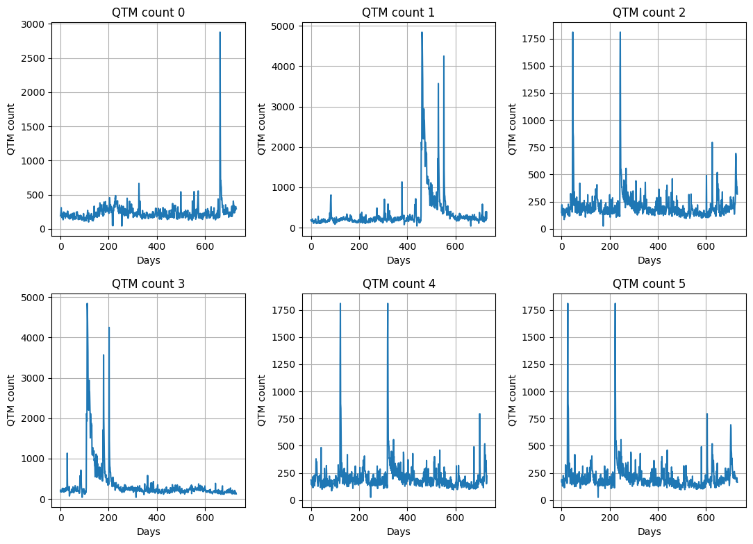
def quick_plot(df_wide,n_timeseries,field="count",dt=1):
    """
    Quick plot of the time series data.

    Parameters:
    df_wide (pd.DataFrame): The wide-format DataFrame containing the time series.
    n_timeseries (int): Number of time series to plot.
    field (str): The field to plot.


    Returns:
    None
    """
    # Determine the number of rows and columns for the subplots
    n_timeseries2 = min(n_timeseries, 6)  # Cap the number of time series to 12
    nrows = (n_timeseries2 - 1) // 3 + 1
    ncols = min(n_timeseries2, 3)

    fig, axes = plt.subplots(nrows=nrows, ncols=ncols, figsize=(11, 8))  # define the figure and subplots
    axes = axes.ravel()
    for i in range(n_timeseries2):
        # create a time axis that multiplies time_data by dt
        # Calculate the time index as the difference from the first datetime
        # df_wide['time_index'] = (df_wide['time_index'] - df_wide['time_index'].iloc[0]).dt.total_seconds() / (24 * 3600)

        # Convert the time_index to a float array
        time_index_days_float = df_wide['time_index'].values


      
        ax = axes[i]
        ax.plot(time_index_days_float, df_wide[f"target_{i+1}"], label=f"{field}_{i+1}")
        ax.set_title(f"{field} {i}")
        ax.set_xlabel("Days")
        ax.set_ylabel(field)
        plt.tight_layout()
        ax.grid()

    plt.show()

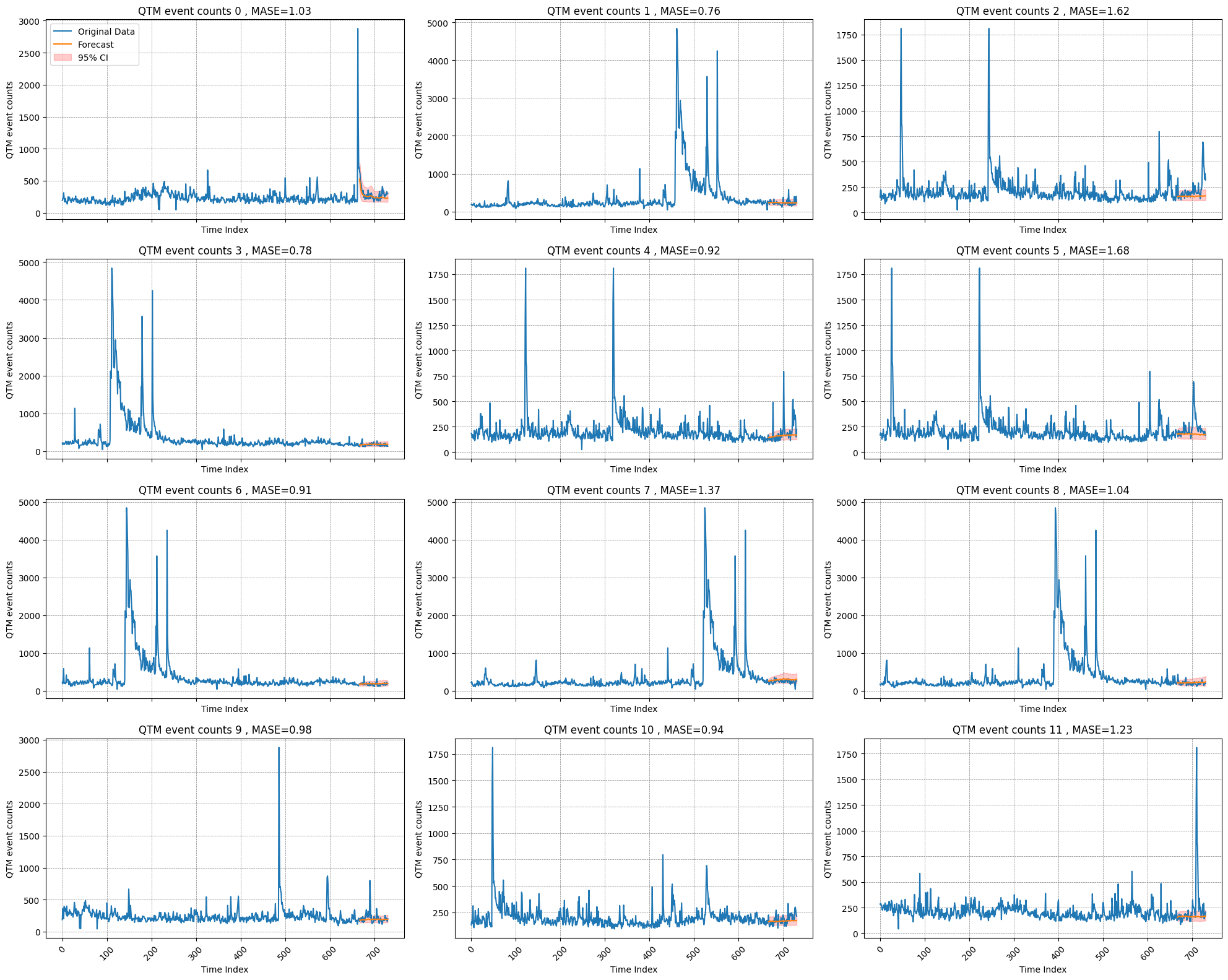
5.1 Earthquake Data#

# first we load data/data_qtm_catalog.csv
df = pd.read_csv("../data/data_qtm_catalog.csv")
df.head()

	datetime	count
0	2008-01-01	120
1	2008-01-02	89
2	2008-01-03	146
3	2008-01-04	166
4	2008-01-05	94

# calculate the time difference between each datetime to set up the dt
# convert the datetime column to datetime object
df["datetime"] = pd.to_datetime(df["datetime"])
dt = df["datetime"].diff().dt.total_seconds().fillna(0).mean()
# convert seconds to days
dt = np.ceil(dt / (60 * 60 * 24))
print(dt)

1.0

Reshape for Prediction#

# randomly cut the long time series into n_timeseries, stored in data frames.
df_list,df_wide = reshape_time_series(df, name_of_target="count", n_timeseries=n_timeseries, duration_years=2)

sampling rate 1.00 days

quick_plot(df_wide,n_timeseries,field="QTM count",dt=1)

../_images/mlgeo_4.10_timeseriesforecast_39_0.png

Predict with Chronos & Plot#

forecast, mean_mae, mean_mase, no_var_mae, split_index = predict_chronos(df_wide,n_timeseries=n_timeseries)
# plot forecast
plot_forecasts(df_wide,split_index,forecast,n_timeseries,field="QTM event counts",filename="./plots/quake_qtm_forecast.png")
# save a vectorized plot

Mean Absolute Error (MAE) for target_1: 48.48504137992859
Mean Absolute Error (MAE) for target_2: 50.47730255126953
Mean Absolute Error (MAE) for target_3: 73.13016510009766
Mean Absolute Error (MAE) for target_4: 29.68954849243164
Mean Absolute Error (MAE) for target_5: 65.26891136169434
Mean Absolute Error (MAE) for target_6: 68.76318144798279
Mean Absolute Error (MAE) for target_7: 35.08878254890442
Mean Absolute Error (MAE) for target_8: 57.32973098754883
Mean Absolute Error (MAE) for target_9: 45.120017528533936
Mean Absolute Error (MAE) for target_10: 53.568915605545044
Mean Absolute Error (MAE) for target_11: 37.61477780342102
Mean Absolute Error (MAE) for target_12: 110.07398819923401
Mean Absolute Error (MAE) for target_13: 39.093090534210205
Mean Absolute Error (MAE) for target_14: 80.03271508216858
Mean Absolute Error (MAE) for target_15: 67.37908172607422
Mean Absolute Error (MAE) for target_16: 43.82308888435364
Mean Absolute Error (MAE) for target_17: 192.06181573867798
Mean Absolute Error (MAE) for target_18: 32.19101405143738
Mean Absolute Error (MAE) for target_19: 41.79396343231201
Mean Absolute Error (MAE) for target_20: 69.41318273544312
Mean of forecast MAEs = 62.019915759563446
Mean Absolute Scaled Error (MASE) for target_1: 1.0329920889196824
Mean Absolute Scaled Error (MASE) for target_2: 0.7644399184447067
Mean Absolute Scaled Error (MASE) for target_3: 1.615994528693845
Mean Absolute Scaled Error (MASE) for target_4: 0.7835951215011284
Mean Absolute Scaled Error (MASE) for target_5: 0.9174344970519285
Mean Absolute Scaled Error (MASE) for target_6: 1.675205116482179
Mean Absolute Scaled Error (MASE) for target_7: 0.9149806707702726
Mean Absolute Scaled Error (MASE) for target_8: 1.3712122445769082
Mean Absolute Scaled Error (MASE) for target_9: 1.037809822671646
Mean Absolute Scaled Error (MASE) for target_10: 0.9770821317745623
Mean Absolute Scaled Error (MASE) for target_11: 0.9411163628338063
Mean Absolute Scaled Error (MASE) for target_12: 1.2275909464598587
Mean Absolute Scaled Error (MASE) for target_13: 0.7725422533422971
Mean Absolute Scaled Error (MASE) for target_14: 0.9836248634757355
Mean Absolute Scaled Error (MASE) for target_15: 1.2271992335191315
Mean Absolute Scaled Error (MASE) for target_16: 0.8978388942160257
Mean Absolute Scaled Error (MASE) for target_17: 1.1899974814650582
Mean Absolute Scaled Error (MASE) for target_18: 1.251872768667009
Mean Absolute Scaled Error (MASE) for target_19: 1.2067001357633624
Mean Absolute Scaled Error (MASE) for target_20: 1.5479754025957226
Mean of forecast MAEs = 1.1168602241612433
Mean of ARIMA MAEs = 97.278125
torch.Size([20, 9, 64])
torch.Size([20, 64])
Mean of forecast MASEs = 1.1049544541817105
12

../_images/mlgeo_4.10_timeseriesforecast_41_1.png

df_wide.head()

	time_index	target_1	target_2	target_3	target_4	target_5	target_6	target_7	target_8	target_9	...	forecast_2	forecast_3	forecast_4	forecast_5	forecast_6	forecast_7	forecast_8	forecast_9	forecast_10	forecast_11
0	0	193	191.0	149.0	216.0	185.0	168.0	223.0	220.0	175.0	...	NaN	NaN	NaN	NaN	NaN	NaN	NaN	NaN	NaN	NaN
1	1	212	180.0	220.0	173.0	176.0	190.0	188.0	246.0	150.0	...	NaN	NaN	NaN	NaN	NaN	NaN	NaN	NaN	NaN	NaN
2	2	250	183.0	220.0	218.0	142.0	171.0	368.0	205.0	181.0	...	NaN	NaN	NaN	NaN	NaN	NaN	NaN	NaN	NaN	NaN
3	3	312	155.0	123.0	199.0	172.0	173.0	588.0	159.0	176.0	...	NaN	NaN	NaN	NaN	NaN	NaN	NaN	NaN	NaN	NaN
4	4	242	184.0	163.0	177.0	146.0	128.0	202.0	153.0	207.0	...	NaN	NaN	NaN	NaN	NaN	NaN	NaN	NaN	NaN	NaN

5 rows × 33 columns

!pip install statsmodels
import statsmodels.api as sm
from statsmodels.tsa.arima.model import ARIMA

Requirement already satisfied: statsmodels in /home/mdenolle/miniconda/envs/quake_chronos_moirai/lib/python3.11/site-packages (0.14.2)
Requirement already satisfied: numpy>=1.22.3 in /home/mdenolle/miniconda/envs/quake_chronos_moirai/lib/python3.11/site-packages (from statsmodels) (1.26.4)
Requirement already satisfied: scipy!=1.9.2,>=1.8 in /home/mdenolle/miniconda/envs/quake_chronos_moirai/lib/python3.11/site-packages (from statsmodels) (1.11.4)
Requirement already satisfied: pandas!=2.1.0,>=1.4 in /home/mdenolle/miniconda/envs/quake_chronos_moirai/lib/python3.11/site-packages (from statsmodels) (2.1.4)
Requirement already satisfied: patsy>=0.5.6 in /home/mdenolle/miniconda/envs/quake_chronos_moirai/lib/python3.11/site-packages (from statsmodels) (0.5.6)
Requirement already satisfied: packaging>=21.3 in /home/mdenolle/miniconda/envs/quake_chronos_moirai/lib/python3.11/site-packages (from statsmodels) (24.1)
Requirement already satisfied: python-dateutil>=2.8.2 in /home/mdenolle/miniconda/envs/quake_chronos_moirai/lib/python3.11/site-packages (from pandas!=2.1.0,>=1.4->statsmodels) (2.9.0.post0)
Requirement already satisfied: pytz>=2020.1 in /home/mdenolle/miniconda/envs/quake_chronos_moirai/lib/python3.11/site-packages (from pandas!=2.1.0,>=1.4->statsmodels) (2024.1)
Requirement already satisfied: tzdata>=2022.1 in /home/mdenolle/miniconda/envs/quake_chronos_moirai/lib/python3.11/site-packages (from pandas!=2.1.0,>=1.4->statsmodels) (2024.1)
Requirement already satisfied: six in /home/mdenolle/miniconda/envs/quake_chronos_moirai/lib/python3.11/site-packages (from patsy>=0.5.6->statsmodels) (1.16.0)

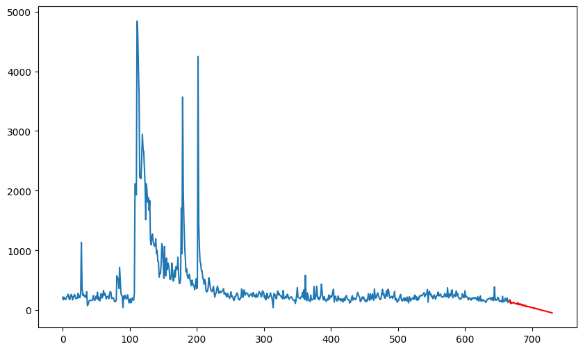
# benchmarking with ARIMA
# Fit ARIMA model
data = df_wide['target_4'][:split_index]
model = ARIMA(data, order=(25, 2, 0))  # (p, d, q) order, adjust as needed
model_fit = model.fit()

# Make predictions
forecast_steps = 64  # Number of steps to forecast
forecast = model_fit.forecast(steps=forecast_steps)

split_index = len(df_wide['target_3'].values) - 64
print(forecast) 
# calculate the MASE between the forecast and the evaluation data
mase=[]
eval_data = df_wide['target_1'][split_index:]
print(len(df_wide['target_1'].values[split_index:]))
# Calculate and print the MASE for each time series
mase.append(np.mean(np.abs(forecast - df_wide['target_1'].values[split_index:])) / np.mean(np.abs(df_wide['target_1'].values[1:] - df_wide['target_1'].values[:-1])))
# print mase
print(f'Mean Absolute Scaled Error (MASE) for ARIMA: {mase[-1]}')

                 

# Plot the results
plt.figure(figsize=(10, 6))
plt.plot(data, label='Actual')
plt.plot(forecast, label='Forecast', color='red')

  170.875002
  109.156006
  134.097091
  115.263988
  123.108176
          ...    
  -36.171929
  -35.465038
  -41.488969
  -41.760654
  -47.384863
Name: predicted_mean, Length: 64, dtype: float64
64
Mean Absolute Scaled Error (MASE) for ARIMA: 4.420838227473031

[<matplotlib.lines.Line2D at 0x7fdd04707e90>]

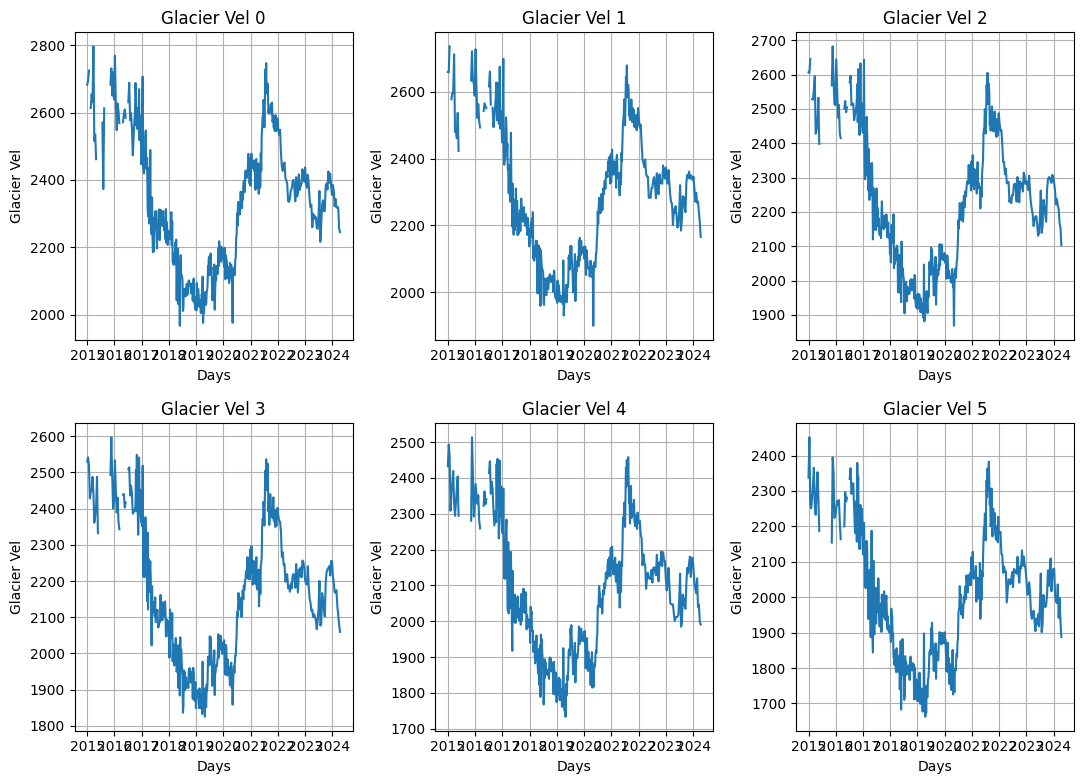
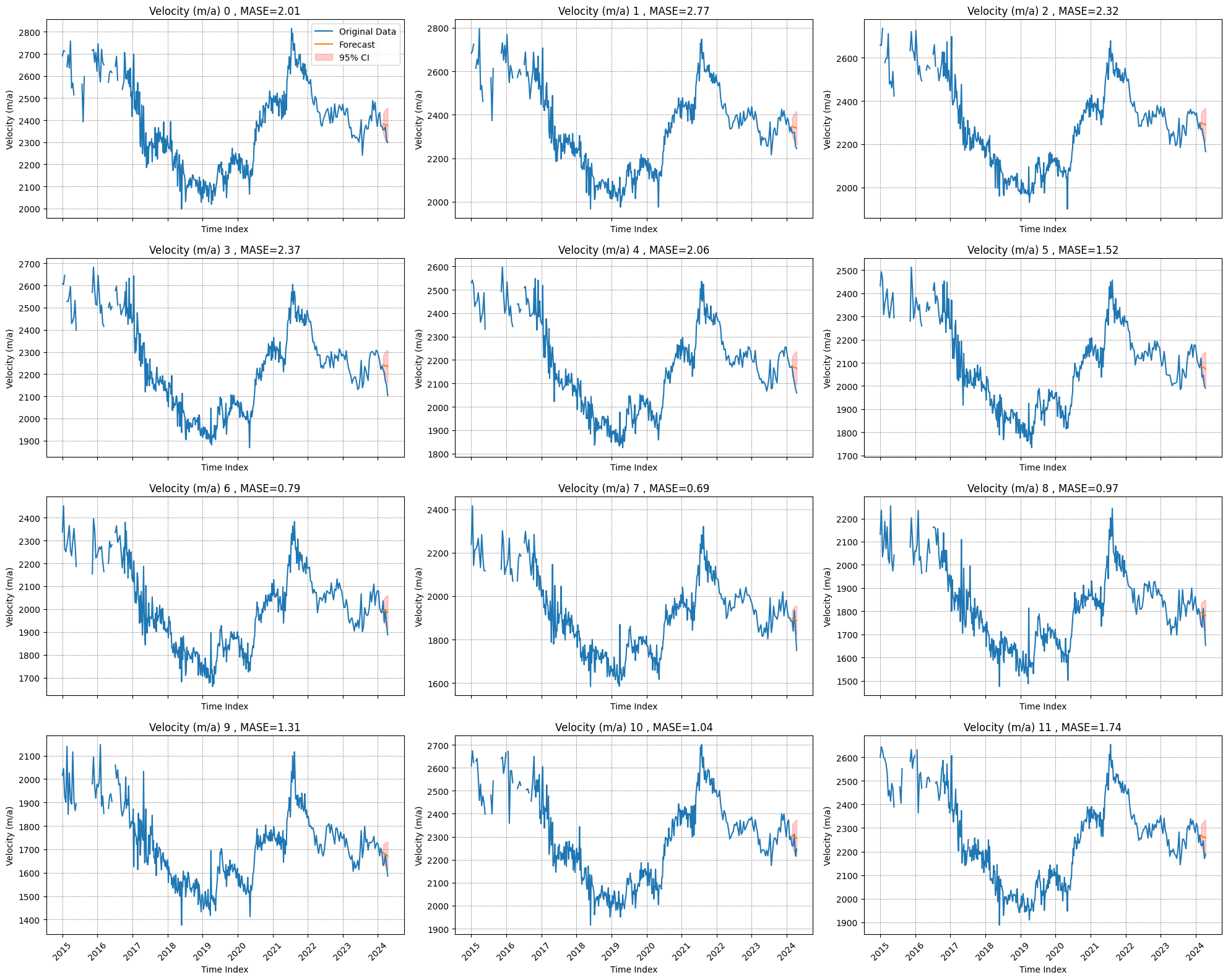
../_images/mlgeo_4.10_timeseriesforecast_44_2.png

5.2 Icesheet velocities#

Now we test the time series of icesheet velocities in Greenland. This is work done by Brad Lipovsky.

'''
Read the data
'''
df = pd.read_csv('../data/data_ice_jakobshavn.csv',na_values=[-1])

# calculate the time difference between each datetime to set up the dt
# convert the datetime column to datetime object
df["datetime"] = pd.to_datetime(df["Date"])
dt = df["datetime"].diff().dt.total_seconds().fillna(0).mean()
# convert seconds to days
dt = np.ceil(dt / (60 * 60 * 24))
print("sampling rate {} days".format(dt))

sampling rate 8.0 days

Reshape for prediction#

df_wide = df
df_wide.dropna()

	Date	Pixel Value (x=2500, y=8200)	Pixel Value (x=2500, y=8201)	Pixel Value (x=2500, y=8202)	Pixel Value (x=2500, y=8203)	Pixel Value (x=2500, y=8204)	Pixel Value (x=2500, y=8205)	Pixel Value (x=2500, y=8206)	Pixel Value (x=2500, y=8207)	Pixel Value (x=2500, y=8208)	...	Pixel Value (x=2509, y=8201)	Pixel Value (x=2509, y=8202)	Pixel Value (x=2509, y=8203)	Pixel Value (x=2509, y=8204)	Pixel Value (x=2509, y=8205)	Pixel Value (x=2509, y=8206)	Pixel Value (x=2509, y=8207)	Pixel Value (x=2509, y=8208)	Pixel Value (x=2509, y=8209)	datetime
0	2015-01-01	2690.5570	2682.3616	2658.6174	2606.9355	2530.3400	2432.4604	2337.5603	2238.3130	2131.6187	...	1860.1473	1811.2555	1772.2811	1739.5938	1691.1827	1651.6400	1610.4110	1563.1417	1513.4183	2015-01-01
1	2015-01-13	2714.7678	2694.3774	2657.5322	2604.6094	2541.0916	2492.7390	2451.3862	2415.7693	2235.5337	...	1866.2997	1801.4703	1747.1519	1679.1748	1619.7880	1580.2765	1548.2367	1506.4203	1471.4894	2015-01-13
2	2015-01-25	2712.4210	2724.5880	2735.8308	2645.3513	2518.3074	2460.4731	2262.7056	2141.2844	2034.8848	...	1807.4071	1738.1703	1679.8862	1627.8777	1575.1526	1554.8282	1534.6147	1520.7195	1515.0082	2015-01-25
4	2015-02-18	2641.4170	2613.6772	2577.1538	2528.2330	2444.6372	2356.7375	2280.1716	2216.3354	2187.7751	...	1803.6461	1748.5105	1696.6669	1643.1813	1591.3317	1547.9862	1504.9419	1459.6843	1411.1000	2015-02-18
5	2015-03-02	2695.7231	2654.4783	2596.1223	2527.4956	2450.6010	2383.8125	2317.7700	2231.7078	2069.8728	...	1768.4241	1721.1057	1695.4995	1661.2021	1618.2247	1578.6671	1531.1387	1487.0217	1451.7004	2015-03-02
...	...	...	...	...	...	...	...	...	...	...	...	...	...	...	...	...	...	...	...	...	...
437	2024-02-25	2355.7673	2317.1812	2267.6526	2218.5762	2174.4893	2119.7183	2036.1709	1886.2402	1742.2327	...	1555.8588	1496.1707	1448.4729	1410.3757	1372.7169	1332.9342	1291.7050	1252.8741	1215.6035	2024-02-25
438	2024-03-08	2356.8071	2318.0103	2271.4500	2208.3280	2131.2380	2038.9028	1941.8640	1839.1848	1730.7375	...	1584.8710	1545.4580	1487.4086	1430.3809	1381.1884	1338.1537	1301.4970	1264.5914	1226.1100	2024-03-08
439	2024-03-20	2369.9165	2318.2954	2239.7700	2166.4363	2106.1460	2046.7198	1997.2346	1934.0216	1812.1205	...	1542.8604	1510.4088	1461.9852	1407.3877	1358.6483	1318.0781	1282.2297	1241.4624	1196.6234	2024-03-20
440	2024-04-01	2304.3186	2255.6506	2209.5908	2154.6484	2079.5513	1998.6061	1931.5712	1849.2580	1743.1146	...	1568.9454	1520.7106	1462.4568	1407.1897	1359.1794	1317.0726	1278.7156	1242.9205	1201.6306	2024-04-01
441	2024-04-13	2300.0273	2244.5710	2165.4233	2103.4187	2059.3809	1990.8022	1887.8052	1750.1135	1652.9683	...	1529.3740	1496.3535	1455.9960	1412.7965	1370.8213	1326.9905	1279.7404	1225.2361	1173.2060	2024-04-13

418 rows × 102 columns

# remove the first column and place the last at first position
df_wide = df_wide.drop(columns=["Date"])
cols = df_wide.columns.tolist()
cols = cols[-1:] + cols[:-1]
df_wide = df_wide[cols]

# now rename all Pixel columns to indexes except for the first one
df_wide.columns = ["time_index"] + ["target_"+str(i) for i in range(len(df_wide.columns)-1)]   

quick_plot(df_wide,n_timeseries,field="Glacier Vel",dt=8)

../_images/mlgeo_4.10_timeseriesforecast_52_0.png

torch.cuda.empty_cache()
import gc
gc.collect()

notebook controller is DISPOSED. 

View Jupyter <a href='command:jupyter.viewOutput'>log</a> for further details.

n_predict = 5
time_forecast = n_predict * dt 
print("Forecasting for {} days".format(time_forecast))

Forecasting for 40.0 days

Predict & Plot forecasts with Chronos#

forecast, mean_mae, mean_mase, no_var_mae, split_index = predict_chronos(df_wide,predict_length=n_predict,n_timeseries=n_timeseries)
# plot
plot_forecasts(df_wide,split_index,forecast,n_timeseries,field="Velocity (m/a)",filename="./plots/ice_jakobshavn_forecast.png")

Mean Absolute Error (MAE) for target_0: 42.24474937499999
Mean Absolute Error (MAE) for target_1: 51.846288281250054
Mean Absolute Error (MAE) for target_2: 63.66113656250009
Mean Absolute Error (MAE) for target_3: 68.27394875
Mean Absolute Error (MAE) for target_4: 59.332813359374995
Mean Absolute Error (MAE) for target_5: 54.84119093749996
Mean Absolute Error (MAE) for target_6: 51.02073972656249
Mean Absolute Error (MAE) for target_7: 56.604517070312525
Mean Absolute Error (MAE) for target_8: 60.905154804687484
Mean Absolute Error (MAE) for target_9: 46.845470039062505
Mean Absolute Error (MAE) for target_10: 45.993564921874984
Mean Absolute Error (MAE) for target_11: 51.39334015625
Mean Absolute Error (MAE) for target_12: 63.96544187500003
Mean Absolute Error (MAE) for target_13: 71.486827890625
Mean Absolute Error (MAE) for target_14: 67.60769390625
Mean Absolute Error (MAE) for target_15: 68.74598835937499
Mean Absolute Error (MAE) for target_16: 62.17083863281255
Mean Absolute Error (MAE) for target_17: 65.56442820312505
Mean Absolute Error (MAE) for target_18: 66.02327011718754
Mean Absolute Error (MAE) for target_19: 64.03354175781246
Mean of forecast MAEs = 59.12804723632813
Mean Absolute Scaled Error (MASE) for target_0: 2.010735538753725
Mean Absolute Scaled Error (MASE) for target_1: 2.7710987795736437
Mean Absolute Scaled Error (MASE) for target_2: 2.3186581656485306
Mean Absolute Scaled Error (MASE) for target_3: 2.3714981221370772
Mean Absolute Scaled Error (MASE) for target_4: 2.0618065531055927
Mean Absolute Scaled Error (MASE) for target_5: 1.5175690902323826
Mean Absolute Scaled Error (MASE) for target_6: 0.7876400007342528
Mean Absolute Scaled Error (MASE) for target_7: 0.6949596678740014
Mean Absolute Scaled Error (MASE) for target_8: 0.966631879403238
Mean Absolute Scaled Error (MASE) for target_9: 1.3144366326702754
Mean Absolute Scaled Error (MASE) for target_10: 1.0350373126193724
Mean Absolute Scaled Error (MASE) for target_11: 1.7442638916464657
Mean Absolute Scaled Error (MASE) for target_12: 3.2202381431841833
Mean Absolute Scaled Error (MASE) for target_13: 2.6931039274055864
Mean Absolute Scaled Error (MASE) for target_14: 2.29931356317334
Mean Absolute Scaled Error (MASE) for target_15: 2.0899756897892243
Mean Absolute Scaled Error (MASE) for target_16: 1.4075847948663025
Mean Absolute Scaled Error (MASE) for target_17: 1.3198358208382497
Mean Absolute Scaled Error (MASE) for target_18: 1.4886333326686638
Mean Absolute Scaled Error (MASE) for target_19: 2.2221349867240554
Mean of forecast MAEs = 1.8167577946524083
Mean of ARIMA MAEs = 55.618072
torch.Size([20, 9, 5])
torch.Size([20, 5])
Mean of forecast MASEs = 1.6328613028665464
12

../_images/mlgeo_4.10_timeseriesforecast_56_1.png

# benchmarking with ARIMA
# Fit ARIMA model
data = df_wide['target_3'][:split_index]
model = ARIMA(data, order=(5, 2, 1))  # (p, d, q) order, adjust as needed
model_fit = model.fit()

# Make predictions
forecast_steps = 64  # Number of steps to forecast
forecast = model_fit.forecast(steps=forecast_steps)

split_index = len(df_wide['target_3'].values) - 64
print(forecast) 
# calculate the MASE between the forecast and the evaluation data
mase=[]
eval_data = df_wide['target_1'][split_index:]
print(len(df_wide['target_1'].values[split_index:]))
# Calculate and print the MASE for each time series
mase.append(np.mean(np.abs(forecast - df_wide['target_1'].values[split_index:])) / np.mean(np.abs(df_wide['target_1'].values[1:] - df_wide['target_1'].values[:-1])))
# print mase
print(f'Mean Absolute Scaled Error (MASE) for ARIMA: {mase[-1]}')

                 

# Plot the results
plt.figure(figsize=(10, 6))
plt.plot(data, label='Actual')
plt.plot(forecast, label='Forecast', color='red')

5.3 Forecasting GPS velocities#

In this case, we are going to test Chrono’s performance on GPS time series. Vertical components tend to exhibit seasonal loading from precipitation, horizontal components tend to exhibit tectonic processes, especially at plate boundaries.

# read data from data_gps_P395_relateive_position.csv
fname = "../data/data_gps_P395_relative_position.csv"
df = pd.read_csv(fname)
# convert dacimal year column to floats
df["decimal year"] = df["decimal year"].astype(float)
df.head()

# the date format is in decimal years, convert it to datetime
# df["datetime"] = pd.to_datetime(df["decimal year"], format="%Y.%j")
# df.head()


# perform a running mean average to smooth the data
for ikey in df.keys()[1:]:
    df[ikey]=df[ikey].rolling(window=20).mean()

sta_name = fname.split("/")[-1].split("_")[2]
print(sta_name)

# take the first column "decimal year" and convert it to a datetime by taking the year before the comma, then multuply by 365.25 to get the days
df["datetime"] = pd.to_datetime((df["decimal year"] - 1970) * 365.25, unit='D', origin='1970-01-01')
# move the last to the first position
cols = df.columns.tolist()
cols = cols[-1:] + cols[:-1]
df = df[cols]
df.head()

df_list,df_wide = reshape_time_series(df,name_of_target="new delta v (m)", n_timeseries=n_timeseries, duration_years=4)
# now predict with chronos
forecast, mean_mae, mean_mase, no_var_mae, split_index = predict_chronos(df_wide,n_timeseries=n_timeseries)
# plot the forecast
plot_forecasts(df_wide,split_index,forecast,n_timeseries,field="GPS relative position (m)",filename="./plots/gps_"+sta_name+"_v_forecast.png")

Horizontal components#

df_list,df_wide = reshape_time_series(df,name_of_target="new delta e (m)", n_timeseries=n_timeseries, duration_years=2)
# now predict with chronos
forecast, mean_mae, mean_mase, no_var_mae, split_index = predict_chronos(df_wide,n_timeseries=n_timeseries)
# plot the forecast
plot_forecasts(df_wide,split_index,forecast,n_timeseries,field="GPS relative position (m)",filename="./plots/gps_"+sta_name+"_e_forecast.png")

torch.cuda.empty_cache()
import gc
gc.collect()

5.4 Forecast dv/v#

# read one dv/v file
fname = "../data/DVV_data_withMean/Data_BGU.csv"
df = pd.read_csv(fname)
df.head()
sta_name = fname.split("/")[-1].split("_")[1]

# convert the date into a timestamp
df["datetime"] = pd.to_datetime(df["date"])
# move datetime to the first position
cols = df.columns.tolist()
cols = cols[-1:] + cols[:-1]
df = df[cols]

5.5 Soil moisture#

df_list,df_wide = reshape_time_series(df,name_of_target="sm_ewt", n_timeseries=n_timeseries, duration_years=4)
# now predict with chronos
forecast, mean_mae, mean_mase, no_var_mae, split_index = predict_chronos(df_wide,n_timeseries=n_timeseries)
# plot the forecast
plot_forecasts(df_wide,split_index,forecast,n_timeseries,field="Soil Moisture",filename="./plots/"+sta_name+"_SM_forecast.png")

df.keys()

for ikey in df.keys()[2:]:
    if ikey == "lake":
        # remove mean of the column
        df[ikey] = df[ikey] - df[ikey].mean()
    df_list,df_wide = reshape_time_series(df,name_of_target=ikey, n_timeseries=n_timeseries, duration_years=4)
    # now predict with chronos
    forecast, mean_mae, mean_mase, no_var_mae, split_index = predict_chronos(df_wide,n_timeseries=n_timeseries)
    # plot the forecast
    plot_forecasts(df_wide,split_index,forecast,n_timeseries,field=ikey,filename="./plots/"+sta_name+"_"+ikey+"_forecast.png")

torch.cuda.empty_cache()
import gc
gc.collect()

5.6 Seismic Wave#

# read CSV file with waveforms in them
df = pd.read_csv("../data/data_waveforms.csv")
df.head()

# trim data between 100 and 200 rows
df = df.iloc[300:500]
plt.plot(df['time'],df['Z'])

#make a datetime column
df["datetime"] = pd.to_datetime(df["time"], unit='s')

df.head()

df_wide.head()

df_wide = df
# rename the keys from Z, N, E, to target_0, target_1, target_2
df_wide.columns = ["time","target_0","target_1","target_2","datetime"]

# reset df_wide index:
df_wide = df_wide.reset_index(drop=True)

# create a time_index column that is the index of the time series
df_wide["time_index"] = np.arange(len(df_wide))

# move datetime to the first position
cols = df_wide.columns.tolist()
cols = cols[-1:] + cols[:-1]
df_wide = df_wide[cols]

# drop columns time and datetime
df_wide = df_wide.drop(columns=["time","datetime"])

# # now predict with chronos
forecast, mean_mae, mean_mase, no_var_mae, split_index = predict_chronos(df_wide,predict_length=64, n_timeseries=len(df.keys())-1)
# # plot the forecast
plot_forecasts(df_wide,split_index,forecast,len(df.keys())-1,field="wave",filename="./plots/waveforms_forecast.png")

# normalize the target data in df_wide to see if this is the problem

df_wide_norm = df_wide.copy()
for ikey in df_wide.keys():
    if ikey != "time_index":
        df_wide_norm[ikey] = (df_wide[ikey] - df_wide[ikey].mean()) / df_wide[ikey].std()


# # now predict with chronos
forecast, mean_mae, mean_mase, no_var_mae, split_index = predict_chronos(df_wide_norm,predict_length=64, n_timeseries=len(df.keys())-1)
# # plot the forecast
plot_forecasts(df_wide_norm,split_index,forecast,len(df.keys())-1,field="wave",filename="./plots/waveforms_forecast_norm.png")

torch.cuda.empty_cache()
import gc
gc.collect()

5.7 CO2#

Here we plan to forecast CO2.

from datetime import datetime, timedelta
fname = "../data/cleaned_data_co2.csv"
df_co2 = pd.read_csv(fname)


# Function to convert decimal year to datetime
def decimal_year_to_datetime(decimal_year):
    year = int(decimal_year)
    remainder = decimal_year - year
    start_of_year = datetime(year, 1, 1)
    days_in_year = (datetime(year + 1, 1, 1) - start_of_year).days
    return start_of_year + timedelta(days=remainder * days_in_year)

# Apply the function to the 'decimale-date' column
df_co2["datetime"] = df_co2["decimale-date"].apply(decimal_year_to_datetime)


# df_co2["datetime"] = pd.to_datetime((df_co2["decimale-date"] - 1970) * 365.25, origin='1970-01-01', unit='D')
df_co2.head()
# # move datetime to the first position
cols = df_co2.columns.tolist()
cols = cols[-1:] + cols[:-1]
df_co2 = df_co2[cols]
df_co2.head()

df_list,df_wide = reshape_time_series(df_co2,name_of_target="monthly-average", n_timeseries=n_timeseries, duration_years=20)
# now predict with chronos
forecast, mean_mae, mean_mase, no_var_mae, split_index = predict_chronos(df_wide,n_timeseries=n_timeseries)
# plot the forecast
plot_forecasts(df_wide,split_index,forecast,n_timeseries,field="C02 Moana",filename="./plots/CO2_forecast.png")

5.8 Paleo Climate Benthic D018 time series#

This time series is phenomenal because it shows how the system switches from 100ka cycle to 20-40ka cycles. https://agupubs.onlinelibrary.wiley.com/doi/full/10.1029/2004PA001071

df_benthic = pd.read_csv("../data/cleaned_lr04.csv")
df_benthic.head()

fig=plt.figure(figsize=(15, 6))
plt.plot(df_benthic["Time-(ka)"],df_benthic["Benthic-d18O-(per-mil)"])   
plt.xlabel("Time (ka)")
plt.ylabel("Benthic d18O (per mil)")
plt.title("Benthic d18O vs Time")
plt.grid() 

# add a time_index column to the dataframe
df_benthic["time_index"] = np.arange(len(df_benthic))
# remove Time-(ka) column
df_benthic = df_benthic.drop(columns=["Time-(ka)"])
# move the last to the first position
cols = df_benthic.columns.tolist()
cols = cols[-1:] + cols[:-1]
df_benthic = df_benthic[cols]
df_benthic.head()

df_benthic_copy.describe()

# now predict with chronos
df_benthic_copy = df_benthic.iloc[:len(df_benthic)//3]
# rename benthic-d18O-(per-mil) to target_1
df_benthic_copy = df_benthic_copy.rename(columns={"Benthic-d18O-(per-mil)":"target_1"})
forecast, mean_mae, mean_mase, no_var_mae, split_index = predict_chronos(df_benthic_copy,predict_length=64,n_timeseries=1)
# plot the forecast
plot_forecasts(df_benthic_copy,split_index,forecast,1,field="D018",filename="./plots/d018_forecast.png")

ML Geo Curriculum

4.10 Time Series Forecast

Contents