2.10 Synthetic noise

Generation of Synthetic Noise for Geoscientific Data

1. Introduction

In geosciences, noise can come from various sources such as environmental factors, instrumentation errors, or anthropogenic activities. Understanding and simulating noise is critical for developing robust data processing techniques, testing algorithms, and validating models. By generating synthetic noise, we can create controlled datasets that simulate real-world scenarios, making it easier to refine techniques for filtering, detection, and interpretation.

This lecture explores how to generate synthetic noise for geoscientific data in two cases:

1. 1D Time Series Data: This could represent data such as seismic records, atmospheric pressure, or sea surface temperature.

2. 2D Geospatial Data: This could represent a spatial field, like topographic maps, soil moisture, or temperature distribution across a region. A realistic example is shown at the end for seismological use cases.

Types of Noise

• White Noise: A random signal with constant power spectral density across all frequencies. This type of noise is common in instrumentation errors.

• Pink Noise: A signal with a power spectrum inversely proportional to its frequency, often seen in natural systems like climate data.

• Gaussian Noise: A specific form of white noise with a normal (Gaussian) distribution of values.

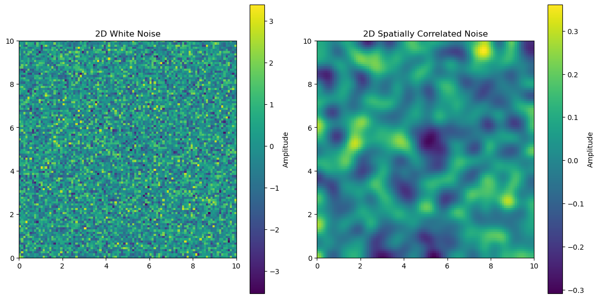
• Spatially Correlated Noise: Noise that varies smoothly over space, often simulating environmental or systematic errors in geospatial datasets.

Use in Geosciences

• In time series data (e.g., seismic signals), synthetic noise is often added to evaluate the effectiveness of filtering and detection algorithms.

• In geospatial datasets, noise can mimic errors introduced by sensors, atmospheric distortions, or spatial smoothing.

1D Time Series Example: Generating White and Pink Noise

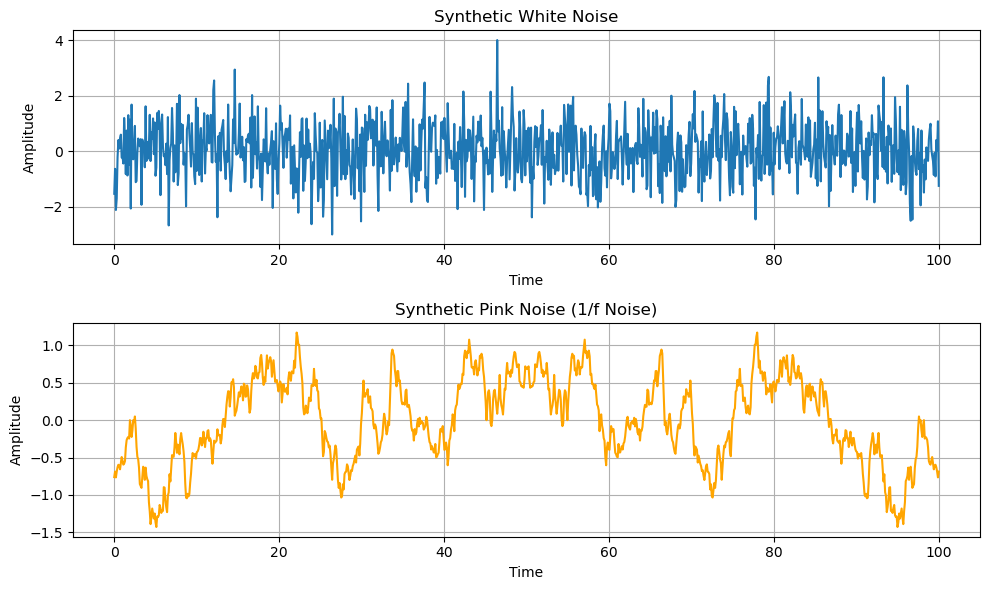
Below is a Python example that demonstrates how to generate and visualize synthetic white and pink noise in a 1D time series, such as for seismic or atmospheric data.

import numpy as np
import matplotlib.pyplot as plt

# Generate synthetic time series (e.g., for seismic or SST data)
n = 1000  # Number of time points
time = np.linspace(0, 100, n)

# Generate white noise (Gaussian distribution)
white_noise = np.random.normal(0, 1, n)

# Generate pink noise (1/f noise)
def generate_pink_noise(size):
    frequencies = np.fft.fftfreq(size)
    pink_spectrum = np.random.normal(size=size) / np.where(frequencies == 0, np.inf, np.abs(frequencies))
    pink_noise = np.fft.ifft(pink_spectrum).real
    return pink_noise

pink_noise = generate_pink_noise(n)

# Plot white noise and pink noise
plt.figure(figsize=(10, 6))

# White noise
plt.subplot(2, 1, 1)
plt.plot(time, white_noise, label='White Noise')
plt.xlabel('Time')
plt.ylabel('Amplitude')
plt.title('Synthetic White Noise')
plt.grid()

# Pink noise
plt.subplot(2, 1, 2)
plt.plot(time, pink_noise, label='Pink Noise', color='orange')
plt.xlabel('Time')
plt.ylabel('Amplitude')
plt.title('Synthetic Pink Noise (1/f Noise)')
plt.grid()

plt.tight_layout()
plt.show()

Explanation:

• White Noise: A time series of Gaussian-distributed random values, which simulates random instrumentation errors.

• Pink Noise: Generated in the frequency domain by applying a 1/f scaling to the frequency components. This noise mimics natural processes, which often exhibit low-frequency dominance.

Applications:

• Seismic Data: White noise can simulate background noise, while pink noise can simulate natural geophysical processes.

• Atmospheric Data: Synthetic noise is added to test filtering techniques for atmospheric time series data, such as removing random disturbances.

2D Geospatial Example: Generating Spatially Correlated Noise

For geospatial data, we often deal with noise that is not purely random but has spatial correlations. This could be due to atmospheric interference or sensor inaccuracies that vary smoothly over space. Below is an example of generating spatially correlated noise in a 2D grid, which might represent a topographic map, temperature distribution, or soil moisture.

import numpy as np
import matplotlib.pyplot as plt
from scipy.ndimage import gaussian_filter

# Generate a 2D grid (e.g., geospatial data, such as a topographic map)
n = 100  # Size of the grid
x = np.linspace(0, 10, n)
y = np.linspace(0, 10, n)
X, Y = np.meshgrid(x, y)

# Generate 2D white noise
white_noise_2d = np.random.normal(0, 1, (n, n))

# Generate spatially correlated noise using a Gaussian filter
spatially_correlated_noise = gaussian_filter(white_noise_2d, sigma=3)

# Plot the synthetic 2D white noise and correlated noise
plt.figure(figsize=(12, 6))

# White noise (unfiltered)
plt.subplot(1, 2, 1)
plt.imshow(white_noise_2d, extent=[0, 10, 0, 10], cmap='viridis')
plt.colorbar(label='Amplitude')
plt.title('2D White Noise')

# Spatially correlated noise
plt.subplot(1, 2, 2)
plt.imshow(spatially_correlated_noise, extent=[0, 10, 0, 10], cmap='viridis')
plt.colorbar(label='Amplitude')
plt.title('2D Spatially Correlated Noise')

plt.tight_layout()
plt.show()

Explanation:

• White Noise in 2D: A random field of Gaussian noise, where each point is independent of the others.

• Spatially Correlated Noise: This noise is generated by applying a Gaussian filter to the white noise, which smooths it and introduces spatial correlations. This simulates real-world noise, such as sensor errors or atmospheric interference that vary smoothly across a geographic region.

Applications:

• Remote Sensing Data: Spatially correlated noise is often introduced into remote sensing images, such as satellite-based soil moisture or temperature data, to simulate atmospheric distortion.

• Topographic Maps: Synthetic noise can simulate measurement errors or interpolation artifacts in spatial datasets like topographic or geophysical maps.

2. Synthetic Noise in Transient Events

Here we will construct a time series with 1 ricker wavelet as a source and synthetic noise

We will analyze their statistical properties and compare the distributions. Present this as a binary classification problem.

import numpy as np
import matplotlib.pyplot as plt
import scipy.signal as sig

fs = 100. # sampling rate
twin = 50. # window length
t = np.linspace(0,twin,int(twin*fs)) #points = 100

1. Event Signal

We will create an event signal as a Ricker wavelet of specified width, 4 seconds in time.

a = 50 # proportional to the width of the wavelet, about a factor of 10
sa = sig.ricker(int(a*fs), a)
# plate the signal in the middle of the time series
s = np.concatenate((np.zeros(len(t)//2-len(sa)//2),sa,np.zeros(len(t)//2-len(sa)//2)))

# plot the signal with nice labels and legends and crispy fonts
plt.figure()
plt.plot(t,s)
plt.xlabel('Time [s]')
plt.ylabel('Amplitude')
plt.grid()
plt.xlim([0,50])
plt.title('Signal')
plt.show()

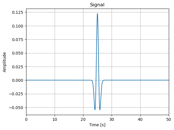
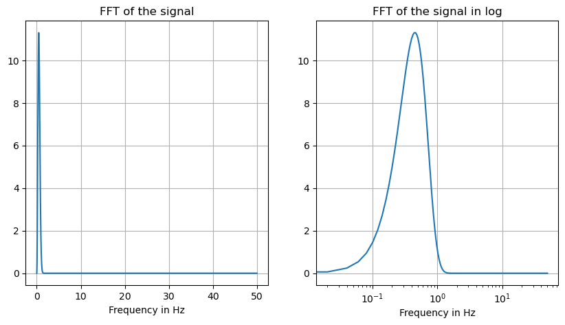
The Ricker wavelet is a smooth function with a signal in a specific frequency band. Let’s plot it’s absolute Fourier amplitude spectrum.

from scipy.fftpack import fft, fftfreq, next_fast_len

## FFT the signals
# fill up until 2^N value to speed up the FFT
Nfft = next_fast_len(len(s)) # this will be an even number

freqVec = fftfreq(Nfft, d=1/fs)[:Nfft//2]
Zhat = fft(s,n=Nfft)

fig,ax=plt.subplots(1,2,figsize=(10,5))
ax[0].plot(freqVec, np.abs(Zhat[:Nfft//2]))
ax[0].grid()
ax[0].set_title('FFT of the signal')
ax[0].set_xlabel('Frequency in Hz')
ax[1].plot(freqVec, np.abs(Zhat[:Nfft//2]))
ax[1].set_xscale('log')
ax[1].set_xlabel('Frequency in Hz')
ax[1].set_title('FFT of the signal in log')
ax[1].grid()

What does the event data distribution looks like?

plt.hist(sa,bins=10)
plt.xlabel('Amplitude')
plt.ylabel('Counts')
plt.title('Histogram of the wavelet')
plt.show()

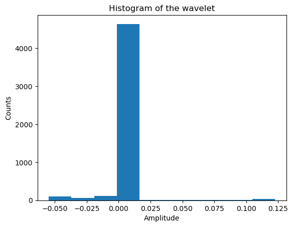
We created a pure signal not contaminated by noise. Let’s create a noise time series to add on the signal time series.

Synthetic noise may take several form.

noise = np.random.rand(len(s))
plt.figure()
plt.plot(t,noise)
plt.xlabel('Time [s]')
plt.ylabel('Amplitude')
plt.grid()
plt.title('Noise')
plt.show()

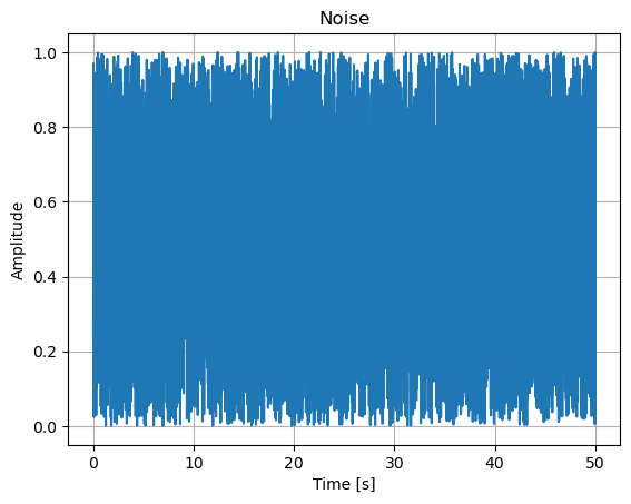
Check the Fourier amplitude spectrum of the noise

nhat = fft(noise,n=Nfft)
plt.plot(freqVec, np.abs(nhat[:Nfft//2]))
plt.plot(freqVec, np.abs(Zhat[:Nfft//2]))
plt.xscale('log')
plt.legend(['noise','signal'])
plt.xlabel('Frequency in Hz')
plt.ylim([0,100])   
plt.grid()

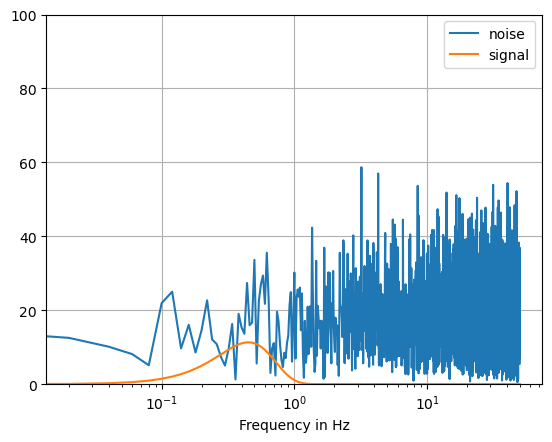
OK, they look very different in the spectral domain! Let’s add noise to the data and plot it.

We will tune a signal to noise ratio to multiply the noise level relative to the signal level. We define this as the max absolute amplitude of the signal, divided by the max absolute amplitude of the noise

SNR = 100 # signal to noise ratio

Now normalize both noise and signal amplitudes.

s /= np.max(np.abs(s)) # normalize the signal
noise /= np.max(np.abs(noise)) # normalize the noise    

noisy_signal = s + noise/SNR
plt.plot(t,noisy_signal)
plt.grid()
plt.title('Noisy signal')
plt.xlabel('Time in s')

Text(0.5, 0, 'Time in s')

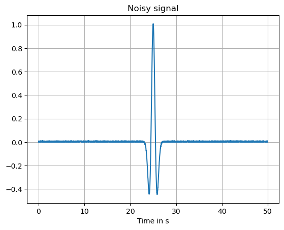
Noise may have different frequency content, or color. We can construct a time series of noise based on its Fourier amplitude spectrum.

from scipy.fftpack import ifft
# random phase
NN = 2*np.pi*np.random.uniform(-1,1,Nfft//2)-np.pi
newnoiseF=np.zeros(Nfft,dtype=np.complex_)
for i in range(Nfft//2):
    newnoiseF[i] = np.exp(1j*NN[i])
    newnoiseF[-i] = np.conj(newnoiseF[i])
newnoiseF[0] = 0
noise = ifft(newnoiseF).real

noise/=np.max(np.abs(noise)) # normalize the noise  
plt.plot(t,noise)
plt.title('Noise with random phase and white spectrum')

Text(0.5, 1.0, 'Noise with random phase and white spectrum')

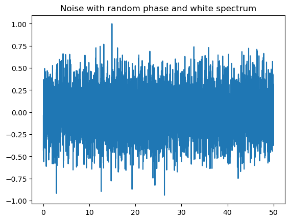
SNR=1

Add the new noise and the signal (Ricker wavelet) and plot them in time and frequency domain

news = s+noise/SNR

fig,ax=plt.subplots(1,2,figsize=(10,5))
ax[0].plot(t,news)
ax[0].set_title('Noisy signal')
ax[0].set_xlabel('Time in s')
ax[0].grid()
ax[1].plot(freqVec, np.abs(fft(news,n=Nfft)[:Nfft//2]))
ax[1].set_xscale('log')
ax[1].grid()
ax[1].set_xlabel('Frequency in Hz')
ax[1].set_title('FFT of the noisy signal in log');

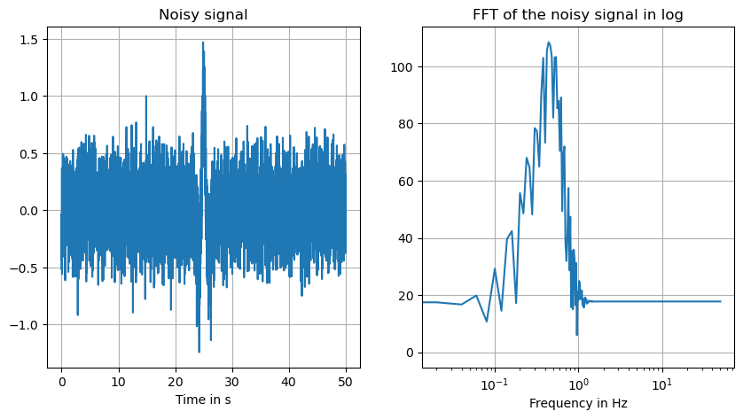
Let’s compare the data distribution between the pure signal, the noise signal, and the combined signals.

fig,ax=plt.subplots(1,2,figsize=(10,5))
ax[0].hist(noise,bins=20);ax[0].grid()
ax[0].hist(s,bins=20);
ax[1].hist(news,bins=20);ax[1].grid();

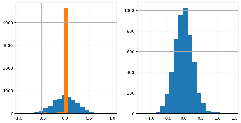
Now in class, calculate the statistical moments between the clean data, the noise, and the noisy data. Explore what features might be discriminate between signal and noise and explore their sensitivity to noise levels.

# calculat statistical moment of the signal
from scipy.stats import moment
print('The first moment of the signal is:',moment(s,1))
print('The second moment of the signal is:',moment(s,2))
print('The third moment of the signal is:',moment(s,3))
print('The fourth moment of the signal is:',moment(s,4))

# calculate the statistical moment of the noise
print('The first moment of the noise is:',moment(noise,1))
print('The second moment of the noise is:',moment(noise,2))
print('The third moment of the noise is:',moment(noise,3))
print('The fourth moment of the noise is:',moment(noise,4))

The first moment of the signal is: 0.0
The second moment of the signal is: 0.0132973926342017
The third moment of the signal is: 0.006434906304516136
The fourth moment of the signal is: 0.007495006078435612
The first moment of the noise is: 0.0
The second moment of the noise is: 0.06302659210056046
The third moment of the noise is: -0.00032277342830262275
The fourth moment of the noise is: 0.01170464605173267

# which moment is the most important for the signal?

4. Realistic or physics-informed synthetic Data and Noise [Level 2]

In this case, we can create a time series that has the similar noise structure than the realistic noise.

These values may mean nothing without some additional context. We can download seismic noise data to see if the earthquake waveforms are statistically different from the noise. For that, we will download the same length of data prior to the earthquake:

!pip install obspy
import obspy
import obspy.clients.fdsn.client as fdsn
from obspy import UTCDateTime 

Requirement already satisfied: obspy in /Users/marinedenolle/opt/miniconda3/envs/mlgeo/lib/python3.9/site-packages (1.4.0)
Requirement already satisfied: numpy>=1.20 in /Users/marinedenolle/opt/miniconda3/envs/mlgeo/lib/python3.9/site-packages (from obspy) (1.26.0)
Requirement already satisfied: scipy>=1.7 in /Users/marinedenolle/opt/miniconda3/envs/mlgeo/lib/python3.9/site-packages (from obspy) (1.11.3)
Requirement already satisfied: matplotlib>=3.3 in /Users/marinedenolle/opt/miniconda3/envs/mlgeo/lib/python3.9/site-packages (from obspy) (3.8.0)
Requirement already satisfied: lxml in /Users/marinedenolle/opt/miniconda3/envs/mlgeo/lib/python3.9/site-packages (from obspy) (4.9.3)
Requirement already satisfied: setuptools in /Users/marinedenolle/opt/miniconda3/envs/mlgeo/lib/python3.9/site-packages (from obspy) (68.2.2)
Requirement already satisfied: sqlalchemy in /Users/marinedenolle/opt/miniconda3/envs/mlgeo/lib/python3.9/site-packages (from obspy) (1.4.49)
Requirement already satisfied: decorator in /Users/marinedenolle/opt/miniconda3/envs/mlgeo/lib/python3.9/site-packages (from obspy) (5.1.1)
Requirement already satisfied: requests in /Users/marinedenolle/opt/miniconda3/envs/mlgeo/lib/python3.9/site-packages (from obspy) (2.31.0)
Requirement already satisfied: contourpy>=1.0.1 in /Users/marinedenolle/opt/miniconda3/envs/mlgeo/lib/python3.9/site-packages (from matplotlib>=3.3->obspy) (1.3.0)
Requirement already satisfied: cycler>=0.10 in /Users/marinedenolle/opt/miniconda3/envs/mlgeo/lib/python3.9/site-packages (from matplotlib>=3.3->obspy) (0.12.0)
Requirement already satisfied: fonttools>=4.22.0 in /Users/marinedenolle/opt/miniconda3/envs/mlgeo/lib/python3.9/site-packages (from matplotlib>=3.3->obspy) (4.43.1)
Requirement already satisfied: kiwisolver>=1.0.1 in /Users/marinedenolle/opt/miniconda3/envs/mlgeo/lib/python3.9/site-packages (from matplotlib>=3.3->obspy) (1.4.5)
Requirement already satisfied: packaging>=20.0 in /Users/marinedenolle/opt/miniconda3/envs/mlgeo/lib/python3.9/site-packages (from matplotlib>=3.3->obspy) (23.2)
Requirement already satisfied: pillow>=6.2.0 in /Users/marinedenolle/opt/miniconda3/envs/mlgeo/lib/python3.9/site-packages (from matplotlib>=3.3->obspy) (10.0.1)
Requirement already satisfied: pyparsing>=2.3.1 in /Users/marinedenolle/opt/miniconda3/envs/mlgeo/lib/python3.9/site-packages (from matplotlib>=3.3->obspy) (3.1.1)
Requirement already satisfied: python-dateutil>=2.7 in /Users/marinedenolle/opt/miniconda3/envs/mlgeo/lib/python3.9/site-packages (from matplotlib>=3.3->obspy) (2.8.2)
Requirement already satisfied: importlib-resources>=3.2.0 in /Users/marinedenolle/opt/miniconda3/envs/mlgeo/lib/python3.9/site-packages (from matplotlib>=3.3->obspy) (6.1.0)
Requirement already satisfied: charset-normalizer<4,>=2 in /Users/marinedenolle/opt/miniconda3/envs/mlgeo/lib/python3.9/site-packages (from requests->obspy) (3.3.0)
Requirement already satisfied: idna<4,>=2.5 in /Users/marinedenolle/opt/miniconda3/envs/mlgeo/lib/python3.9/site-packages (from requests->obspy) (3.4)
Requirement already satisfied: urllib3<3,>=1.21.1 in /Users/marinedenolle/opt/miniconda3/envs/mlgeo/lib/python3.9/site-packages (from requests->obspy) (1.26.20)
Requirement already satisfied: certifi>=2017.4.17 in /Users/marinedenolle/opt/miniconda3/envs/mlgeo/lib/python3.9/site-packages (from requests->obspy) (2023.7.22)
Requirement already satisfied: zipp>=3.1.0 in /Users/marinedenolle/opt/miniconda3/envs/mlgeo/lib/python3.9/site-packages (from importlib-resources>=3.2.0->matplotlib>=3.3->obspy) (3.17.0)
Requirement already satisfied: six>=1.5 in /Users/marinedenolle/opt/miniconda3/envs/mlgeo/lib/python3.9/site-packages (from python-dateutil>=2.7->matplotlib>=3.3->obspy) (1.16.0)

[notice] A new release of pip is available: 23.3.1 -> 24.2
[notice] To update, run: pip install --upgrade pip

# Download seismic data
network = 'UW'
station = 'RATT'
channel = 'HHZ'# this channel gives a low frequency, 1Hz signal.
Tstart = UTCDateTime(2021,7,29,6,15)
fdsn_client = fdsn.Client('IRIS') # client to query the IRIS DMC server
# call to download the specific data: noise waveforms
N = fdsn_client.get_waveforms(network=network, station=station, location='--', channel=channel, starttime=Tstart-7200, \
    endtime=Tstart, attach_response=True)
N.merge(); N.detrend(type='linear');N[0].taper(max_percentage=0.05)

UW.RATT..HHZ | 2021-07-29T04:15:00.000000Z - 2021-07-29T06:14:59.990000Z | 100.0 Hz, 720000 samples

From the Fourier domain, use np.rand[n] functions to create a random phase spectrum between -\(\pi\) and \(\pi\). For the amplitude spectrum, you may choose a white color, which means that the amplitude spectrum is flat and equal at all frequencies; you may choose a color for the spectrum, for instance an amplitude that decays with \(1/f\); you may choose the spectrum of the realistic noise, for instance extracted from raw data.

Random noise

Below, use the random function to create a synthetic noise.

1. Create an array of random numbers between -1 and 1 of length the same length as the data Z.

2. Calculate the signal-to-noise ratio, for instance:

\( SNR = 20 log_{10} (\frac{\max(|signal|)}{\max(|noise|)})\)

or simply

\(SNR = (\frac{\max(|signal|)}{\max(|noise|)})\)

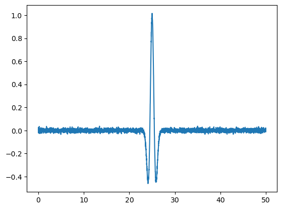
1. Add the synthetic noise with a varying SNR

# 1. Create a time series of the synthetic noise
import numpy.random as random

new_noise= random.randn(len(t))

SNR=100.
plt.plot(t,s/np.max(np.abs(s)) +new_noise/SNR);

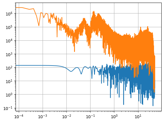
# Make noise based on the spectrum of the noise data
npts = N[0].stats.npts-1
## FFT the signals
# fill up until 2^N value to speed up the FFT
Nfft = next_fast_len(int(N[0].data.shape[0]-1)) # this will be an even number
freqVec = fftfreq(Nfft, d=N[0].stats.delta)[:Nfft//2]
Nat = fft(new_noise,n=Nfft)#/np.sqrt(Z[0].stats.npts)


plt.plot(freqVec,np.abs(Nat[:Nfft//2]))

N.taper(max_percentage=0.05)
Nhat = fft(N[0].data,n=Nfft)#/np.sqrt(Z[0].stats.npts)

plt.plot(freqVec,np.abs(Nhat[:Nfft//2]))
plt.xscale('log');plt.yscale('log');plt.grid()

from scipy.fftpack import ifft
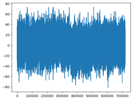
Nhat = fft(N[0].data,n=Nfft)#/np.sqrt(Z[0].stats.npts)
NN = 2*np.pi*random.uniform(-1,1,Nfft//2)-np.pi
newcrap=np.zeros(Nfft,dtype=np.complex_)

for i in range(Nfft//2):
    newcrap[i] = np.abs(Nhat[i])*np.exp(1j*NN[i])
    newcrap[-i] = np.conj(NN[i])
newnoiseF[0] = 0
crap = ifft(newcrap).real
plt.plot(crap)

[<matplotlib.lines.Line2D at 0x16d096220>]

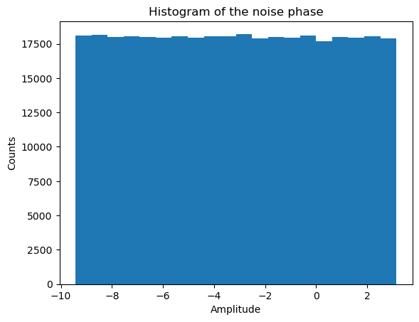
NN = 2*np.pi*random.uniform(-1,1,Nfft//2)-np.pi
# plot a histogram of the noise
plt.hist(NN,bins=20)
plt.xlabel('Amplitude')
plt.ylabel('Counts')
plt.title('Histogram of the noise phase')

Text(0.5, 1.0, 'Histogram of the noise phase')

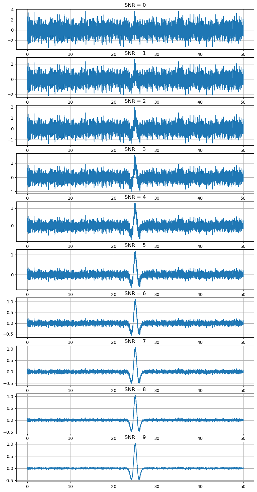
# plot the data over various SNR
# create a figure with 10 subplots as rows
fig,ax = plt.subplots(10,1,figsize=(10,20))
for i,snr in enumerate([np.power(10,i/5) for i in range(10)]):
    ax[i].plot(t,s/np.max(np.abs(s)) +new_noise/snr);
    ax[i].set_title('SNR = '+str(i))
    ax[i].grid()
plt.show()

Exercise

Create synthetic noise for images.