2.5 Data Arrays
Contents
2.5 Data Arrays#
This lecture introduces arrays.
1. Why Manipulate Arrays in Geoscientific Data?#
Data Complexity: Geoscientific data is often multidimensional (e.g., 3D grids for seismic data, 4D climate models with time). Arrays offer efficient ways to store and manipulate such data.
Data Transformation: Preprocessing geoscientific data often involves transformations such as normalization, aggregation, resampling, and feature extraction, all of which require array manipulation.
Performance: Arrays provide optimized data structures that make operations faster and more memory efficient. This is crucial when working with large datasets (e.g., satellite imagery, climate models).
Model Input: Machine learning models, especially deep learning, often require structured data inputs in the form of arrays or tensors.
Overview of Array Libraries
NumPy Arrays: The foundation for numerical computing in Python. Offers basic array operations, efficient mathematical functions, and indexing/slicing tools.
Xarray: Designed for labeled, multi-dimensional data. Xarray is ideal for geoscientific data that has labels for each dimension (e.g., time, latitude, longitude).
PyTorch Tensors: A library primarily for deep learning. It allows for GPU-accelerated tensor operations and is useful when geoscientific problems intersect with machine learning tasks.
At all levels, we will practice
Matplotlib python package that provides functionalities for basic plotting.
2. Numpy arrays#
Sequence of data can be stored in python lists. Lists are very flexible; data of identical type can be appended to list on the fly.
Numpy arrays area multi-dimensional objects of specific data types (floats, strings, integers, …). ! Numpy arrays should be declared first ! Allocating memory of the data ahead of time can save computational time. Numpy arrays support arithmetic operations. There are numerous tutorials to get help. https://www.earthdatascience.org/courses/intro-to-earth-data-science/scientific-data-structures-python/numpy-arrays/
# import module
import numpy as np

# define an array of dimension one from.
#this is a list of floats:
a=[0.7 , 0.75, 1.85]
# convert a list to a numpy array
a_nparray = np.array(a)
2.1 1D arrays in Numpy#
1-D arrays are also called vectors. The Numpy function arange will create regularly spaced values within a specific range. It is similar to the python function range.
# create 1D arrays
N=100
x_int = np.arange(N)# this will make a vector of int from 0 to N-1
print(x_int)
[ 0  1  2  3  4  5  6  7  8  9 10 11 12 13 14 15 16 17 18 19 20 21 22 23
 24 25 26 27 28 29 30 31 32 33 34 35 36 37 38 39 40 41 42 43 44 45 46 47
 48 49 50 51 52 53 54 55 56 57 58 59 60 61 62 63 64 65 66 67 68 69 70 71
 72 73 74 75 76 77 78 79 80 81 82 83 84 85 86 87 88 89 90 91 92 93 94 95
 96 97 98 99]
N = 100 # number of points

# linearly spaced vectors
x_lat = np.linspace(39,50,N)# this will make a vector of floats from min to max values evenly spaced
x_lon = np.linspace(-128,-125,N)# same for longitude
print(x_lat)
print(x_lon)


# logspaced vectors
# 10^(-1) -> 10^(1) => 0.1 - 1
x_tl = np.logspace(-1,1,N)

print(x_tl)
[39.         39.11111111 39.22222222 39.33333333 39.44444444 39.55555556
 39.66666667 39.77777778 39.88888889 40.         40.11111111 40.22222222
 40.33333333 40.44444444 40.55555556 40.66666667 40.77777778 40.88888889
 41.         41.11111111 41.22222222 41.33333333 41.44444444 41.55555556
 41.66666667 41.77777778 41.88888889 42.         42.11111111 42.22222222
 42.33333333 42.44444444 42.55555556 42.66666667 42.77777778 42.88888889
 43.         43.11111111 43.22222222 43.33333333 43.44444444 43.55555556
 43.66666667 43.77777778 43.88888889 44.         44.11111111 44.22222222
 44.33333333 44.44444444 44.55555556 44.66666667 44.77777778 44.88888889
 45.         45.11111111 45.22222222 45.33333333 45.44444444 45.55555556
 45.66666667 45.77777778 45.88888889 46.         46.11111111 46.22222222
 46.33333333 46.44444444 46.55555556 46.66666667 46.77777778 46.88888889
 47.         47.11111111 47.22222222 47.33333333 47.44444444 47.55555556
 47.66666667 47.77777778 47.88888889 48.         48.11111111 48.22222222
 48.33333333 48.44444444 48.55555556 48.66666667 48.77777778 48.88888889
 49.         49.11111111 49.22222222 49.33333333 49.44444444 49.55555556
 49.66666667 49.77777778 49.88888889 50.        ]
[-128.         -127.96969697 -127.93939394 -127.90909091 -127.87878788
 -127.84848485 -127.81818182 -127.78787879 -127.75757576 -127.72727273
 -127.6969697  -127.66666667 -127.63636364 -127.60606061 -127.57575758
 -127.54545455 -127.51515152 -127.48484848 -127.45454545 -127.42424242
 -127.39393939 -127.36363636 -127.33333333 -127.3030303  -127.27272727
 -127.24242424 -127.21212121 -127.18181818 -127.15151515 -127.12121212
 -127.09090909 -127.06060606 -127.03030303 -127.         -126.96969697
 -126.93939394 -126.90909091 -126.87878788 -126.84848485 -126.81818182
 -126.78787879 -126.75757576 -126.72727273 -126.6969697  -126.66666667
 -126.63636364 -126.60606061 -126.57575758 -126.54545455 -126.51515152
 -126.48484848 -126.45454545 -126.42424242 -126.39393939 -126.36363636
 -126.33333333 -126.3030303  -126.27272727 -126.24242424 -126.21212121
 -126.18181818 -126.15151515 -126.12121212 -126.09090909 -126.06060606
 -126.03030303 -126.         -125.96969697 -125.93939394 -125.90909091
 -125.87878788 -125.84848485 -125.81818182 -125.78787879 -125.75757576
 -125.72727273 -125.6969697  -125.66666667 -125.63636364 -125.60606061
 -125.57575758 -125.54545455 -125.51515152 -125.48484848 -125.45454545
 -125.42424242 -125.39393939 -125.36363636 -125.33333333 -125.3030303
 -125.27272727 -125.24242424 -125.21212121 -125.18181818 -125.15151515
 -125.12121212 -125.09090909 -125.06060606 -125.03030303 -125.        ]
1.0101010101010102
[ 0.1         0.10476158  0.10974988  0.1149757   0.12045035  0.12618569
  0.13219411  0.13848864  0.14508288  0.15199111  0.15922828  0.16681005
  0.17475284  0.18307383  0.19179103  0.2009233   0.21049041  0.22051307
  0.23101297  0.24201283  0.25353645  0.26560878  0.27825594  0.29150531
  0.30538555  0.31992671  0.33516027  0.35111917  0.36783798  0.38535286
  0.40370173  0.42292429  0.44306215  0.46415888  0.48626016  0.5094138
  0.53366992  0.55908102  0.58570208  0.61359073  0.64280731  0.67341507
  0.70548023  0.7390722   0.77426368  0.81113083  0.84975344  0.89021509
  0.93260335  0.97700996  1.02353102  1.07226722  1.12332403  1.17681195
  1.23284674  1.29154967  1.35304777  1.41747416  1.48496826  1.55567614
  1.62975083  1.70735265  1.78864953  1.87381742  1.96304065  2.05651231
  2.15443469  2.25701972  2.36448941  2.47707636  2.59502421  2.71858824
  2.84803587  2.98364724  3.12571585  3.27454916  3.43046929  3.59381366
  3.76493581  3.94420606  4.1320124   4.32876128  4.53487851  4.75081016
  4.97702356  5.21400829  5.46227722  5.72236766  5.9948425   6.28029144
  6.57933225  6.8926121   7.22080902  7.56463328  7.92482898  8.30217568
  8.69749003  9.11162756  9.54548457 10.        ]
# time vectors
x_t = np.linspace(0,100,N+1)
dt=x_t[1]
print(dt)
1.0
Indexing Numpy arrays
Accessing individual elements is done using squared brackets []. First element is indexed at 0, last element is indexed at -1.
arr = np.arange(5)

# Access the first element (index 0)
element = arr[0]
print(element)  # Output: 1

# Access the fourth element (index 3)
element = arr[3]
print(element)  # Output: 4


# Access the last element (index 5)
element = arr[4]
print(element)  # Output: 5

# Access the last element (index 5)
element = arr[-1]
print(element)  # Output: 5
0
3
4
4
Slicing
We can slice arrays using the basic syntax start:stop:step:
x=np.arange(10)
print(x)
[0 1 2 3 4 5 6 7 8 9]
# select subarrays between indexes 3 and 6
x1 = x[2:10:2]
print(x1)
[2 4 6 8]
Create an array that select every other elements
# answer here
Create an array with a reversed ordered indexes:
# answer here
x[10:0:-1]
array([9, 8, 7, 6, 5, 4, 3, 2, 1])
2.2 Plotting with Matplotlib#
Some tips from Sofware-Carpentry
Make sure your text is large enough to read. Use the fontsize parameter in
xlabel,ylabel,title, andlegend, andtick_paramswith labelsize to increase the text size of the numbers on your axes.Similarly, you should make your graph elements easy to see. Use
sto increase the size of your scatterplot markers and linewidth to increase the sizes of your plot lines.Using color (and nothing else) to distinguish between different plot elements will make your plots unreadable to anyone who is colorblind, or who happens to have a black-and-white office printer. For lines, the linestyle parameter lets you use different types of lines. For scatterplots, marker lets you change the shape of your points. If you’re unsure about your colors, you can use Coblis or Color Oracle to simulate what your plots would look like to those with colorblindness.
# make the plots appear in the notebook
%matplotlib inline
import matplotlib.pyplot as plt
# import matplotlib.pylab as pylab

# set default parameters
params = {'legend.fontsize': 14, \
          'xtick.labelsize':14, \
          'ytick.labelsize':14, \
          'font.size':14}
plt.rcParams.update(params)
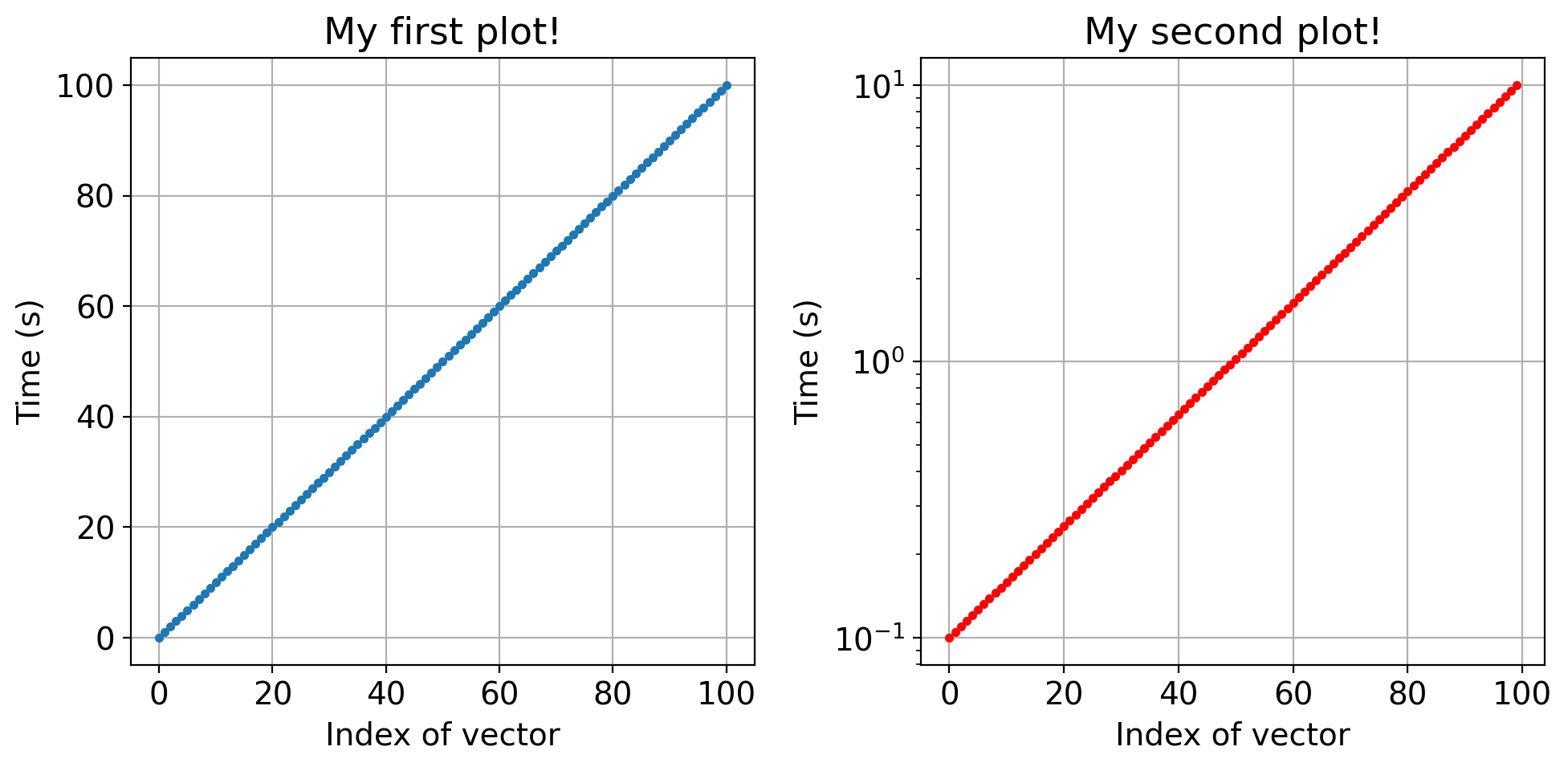
fig, (ax1,ax2) = plt.subplots(1,2, figsize=(10,5))  #
ax1.plot(x_t,'.') # plot the vector x_t
ax2.plot(x_tl,'r.');ax2.set_yscale('log') # plot the vector x_tl in red and log scale
ax2.set_xlabel('Index of vector') # set the x-axis label
ax1.set_xlabel('Index of vector') # set the x-axis label
ax2.set_ylabel('Time (s)') # set the y-axis label
ax1.set_ylabel('Time (s)') # set the y-axis label
ax1.set_title('My first plot!')
ax2.set_title('My second plot!') ;
plt.tight_layout()
ax1.grid(True)
ax2.grid(True)
plt.savefig('plot_test.png')
2.3 Random Arrays#
Creating synthetic arrays from statistical distributions of data.
Find some basic function from the statistics functions in Numpy: https://numpy.org/doc/stable/reference/routines.statistics.html
# generate random fields
from numpy import random

N=10000 # number of samples
# Uniform distribution
x1=2*random.rand(N)-1    # uniform distribution centered at 0, varying between -1 and 2.
# Gaussian distribution
x2=random.randn(N)   # Gaussian distribution with a standard deviation of 1
# Power law
a=2 # power of the distribution
x3=random.power(a,N)
# poisson
aa=4
x4=random.poisson(aa,N)
# now compare this distribution to the Gaussian distribution
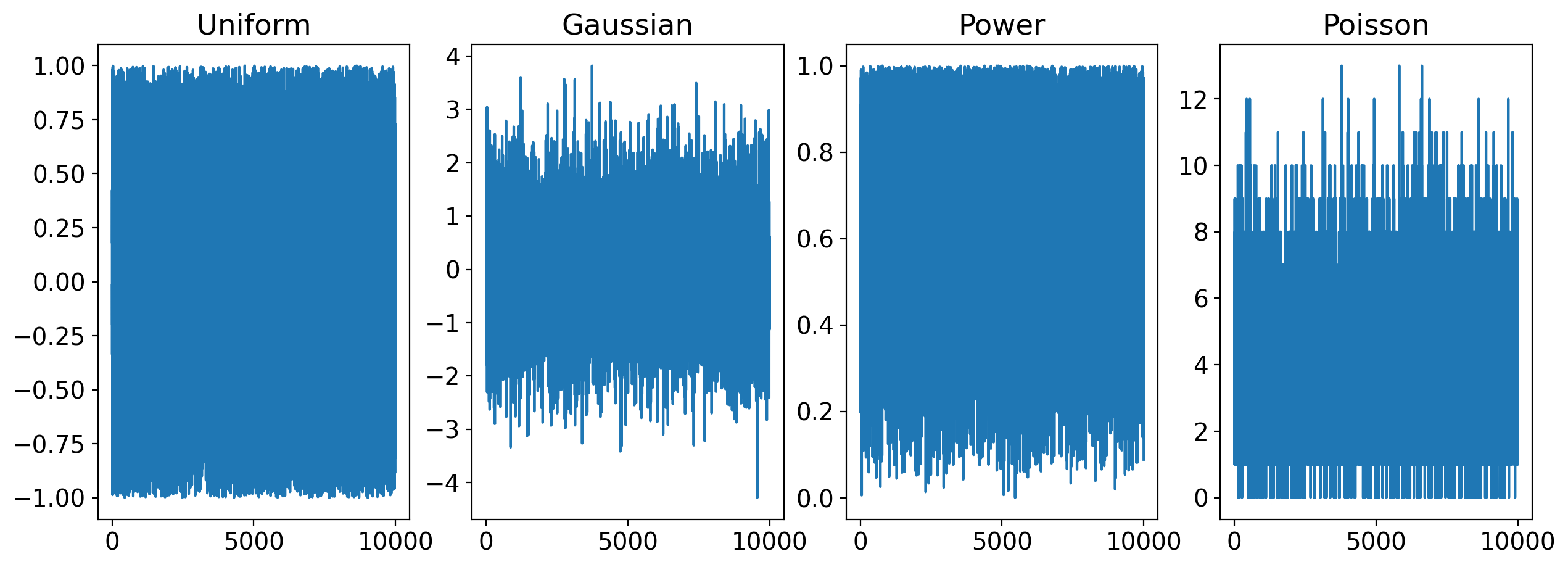
fig1, (ax1,ax2,ax3,ax4) = plt.subplots(1,4, figsize=(15,5))  # 1 row, 2 co
ax1.plot(x1);ax1.set_title('Uniform')
ax2.plot(x2);ax2.set_title('Gaussian')
ax3.plot(x3);ax3.set_title('Power')
ax4.plot(x4);ax4.set_title('Poisson')


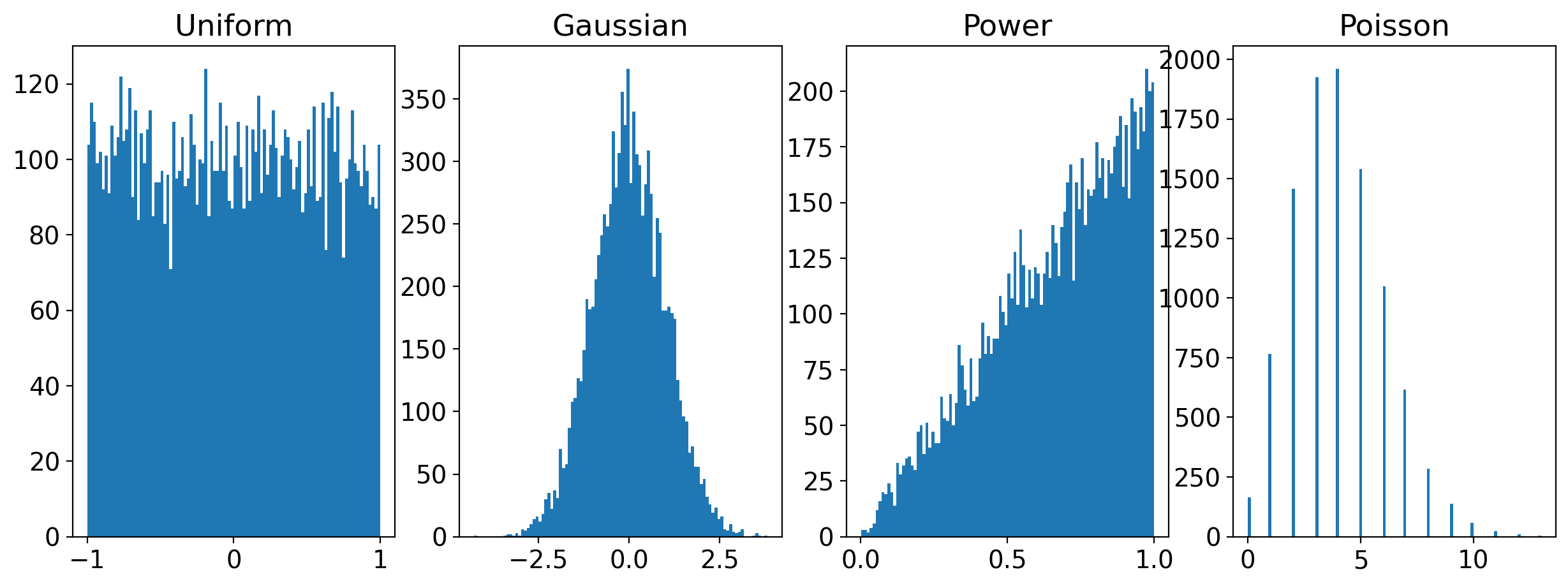
# plot the 2 histograms
fig2, (ax11,ax12,ax13,ax14) = plt.subplots(1,4, figsize=(15,5))  # 1 row, 2 co
ax11.hist(x1,bins=100);ax11.set_title('Uniform')
ax12.hist(x2,bins=100);ax12.set_title('Gaussian')
ax13.hist(x3,bins=100);ax13.set_title('Power')
ax14.hist(x4,bins=100);ax14.set_title('Poisson')
Text(0.5, 1.0, 'Poisson')
# numpy has built-in functions to calculate basic statistical properties of numpy arrays
print("mean of x1", "standard deviation of x1","mean of x2", "standard deviation of x2",)
print(np.mean(x1),np.std(x1),np.mean(x2),np.std(x2))
mean of x1 standard deviation of x1 mean of x2 standard deviation of x2
-0.008060063544843572 0.5777710951796506 0.0009188263163747461 1.0030715920533113
2.4 2D arrays in Numpy#
We will now create random 2D arrays
N=1000 # number of samples
# create
# Uniform distribution
x1=2*random.rand(N,N)-1    # uniform distribution centered at 0, varying between -1 and 2.
# Gaussian distribution
x2=random.randn(N,N)   # Gaussian distribution with a standard deviation of 1
# Power law
a=2 # power of the distribution
x3=random.power(a,[N,N])
# poisson
aa=4
x4=random.poisson(aa,[N,N])

# now compare this distribution to the Gaussian distribution
fig, (ax1,ax2,ax3,ax4) = plt.subplots(1,4, figsize=(26,4))  # 1 row, 2 co
ax1.pcolor(x1,vmin=-1, vmax=1)
ax2.pcolor(x2,vmin=-1, vmax=1)
ax3.pcolor(x3,vmin=-1, vmax=1)
ax4.pcolor(x4,vmin=0, vmax=10)
<matplotlib.collections.PolyQuadMesh at 0x685db3790>

Bonus#
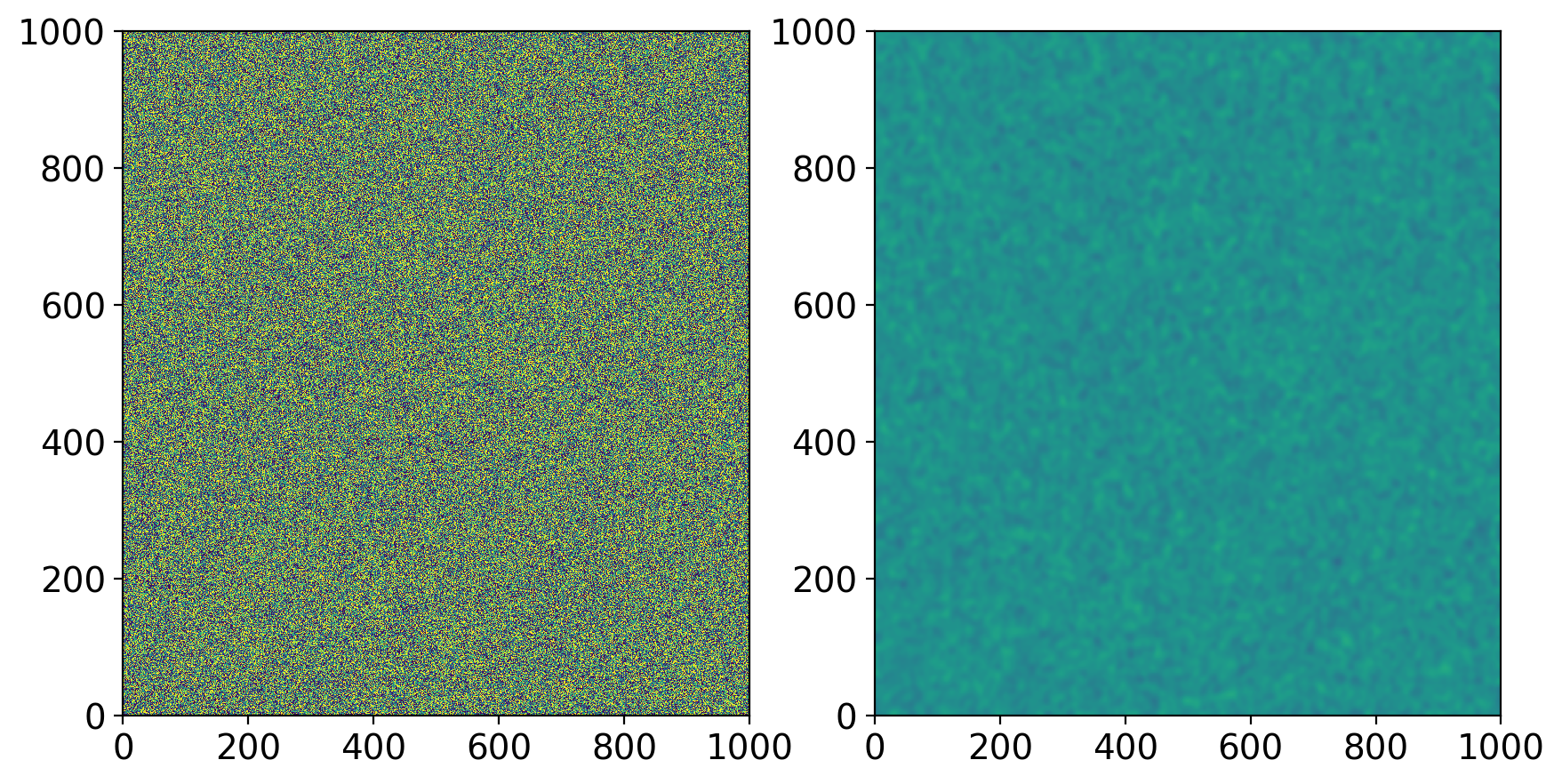
Learn how to smooth/blurr these 2D arrays
# use scipy gaussian filtering to smooth the x2 array
from scipy.ndimage import gaussian_filter
x2_smooth = gaussian_filter(x2, sigma=5)
fig, (ax1,ax2) = plt.subplots(1,2, figsize=(10,5))  # 1 row, 2 co
ax1.pcolor(x2,vmin=-1, vmax=1)
ax2.pcolor(x2_smooth,vmin=-1, vmax=1)
<matplotlib.collections.PolyQuadMesh at 0x78d4ee490>
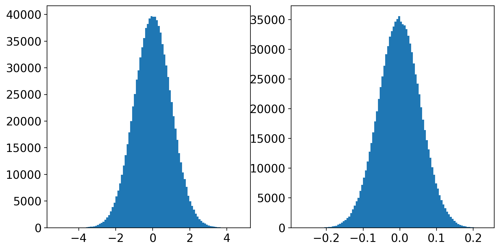
# check the distributions of both arrays before and after smoothing using histograms to compare
fig, (ax1,ax2) = plt.subplots(1,2, figsize=(10,5))  # 1 row, 2 co
ax1.hist(x2.flatten(),bins=100) # flatten the 2D array to 1D and plot the histogram
ax2.hist(x2_smooth.flatten(),bins=100);
2.5 Array Norms#
\(L_2\) norm of an array \(X\):
\(||X||_2 = \sqrt{\sum_i^N \left(X_i^2\right) / N} \)
In numpy that is the default norm of the linear algebra module linalg: np.linalg.norm(X)
We can normalize an array and will focus on wich dimension the array is normalized.
# define random array
x1=2*random.rand(N)-1    # uniform distribution centered at 0, varying between -1 and 2.
# calculate its norm
norm_x1 = np.linalg.norm(x1);print(norm_x1)
# normalize it
x1_norm = x1/norm_x1
# calculate its norm
norm_x1_norm = np.linalg.norm(x1_norm);print(norm_x1_norm)
18.298557385097123
1.0
2.6 Measures of distance#
Comparing data often means calculating a distance or dissimilarity between the two data. Similarity is equialent to proximity of two data.
Euclidian distance
\(L_2\) norm of the residual between 2 vectors:
\(d = ||X -Y||_2 = \sqrt{\sum_i^N \left(X_i^2 - Y_i^2 \right) / N} \)
In numpy that is the default norm of the linear algebra module linalg: d=np.linalg.norm(X-Y)
Total variation distance
Is the \(L_1\)-norm equivalent of the Euclidian distance: d=np.linalg.norm(X-Y,ord=1)
Pearson coefficient (aka the correlation coefficient)
\( P(X,Y) = \frac{cov(X,Y)}{std(X)std(Y)} \)
\( P(X,Y) = \frac{ \sum{ (X_i-mean(X)) (Y_i-mean(Y)}}{\sqrt{\sum{ (X_i-mean(X))^2 } \sum{ (Y_i-mean(Y))^2 } }} \)
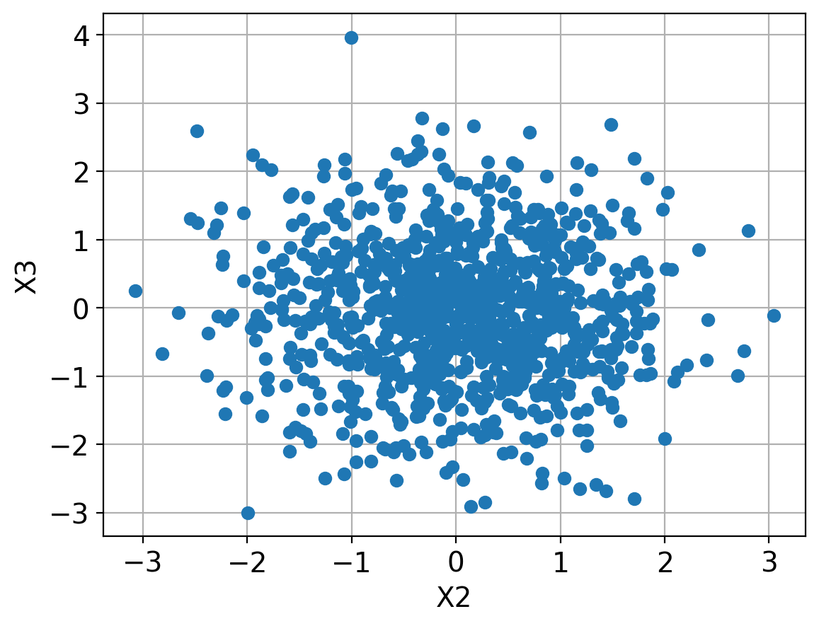
# cross correlate 2 vectors:

x2=random.randn(N)   # Gaussian distribution
x3=random.randn(N)   # Gaussian distribution

# Euclidian distance and make sure it is normalized
d2=np.linalg.norm(x3-x2)    # Euclidian distance
# Total variation distance:
d1=np.linalg.norm(x3-x2,ord=1)
# Pearson coefficient
r = np.corrcoef(x2,x3)[0,1]

# what is the mean of the distances between each point of the two vectors?
dist = np.sqrt(np.sum(np.abs(x3-x2)**2))

print("the three distances are:")
print(d2,d1,r,dist)

plt.plot(x2,x3,'o');plt.grid(True)
plt.xlabel('X2');plt.ylabel('X3')
the three distances are:
45.2937735034487 1136.7159964058294 -0.04303176034198916 45.29377350344869
Text(0, 0.5, 'X3')
3. Xarrays#
3.1 Xarray basics#
This tutorial has been copied and modified from the Xarray package tutorials.
Geoscientific data comes with complex metadata that describe the meaning and context for data arrays. Xarrays allows to attach metadat to the data arrays, making it easier to keep track of variables, their units, coordinate systems, and other important data attributes. Because geoscientific data are typically multi-dimensional, integrating dimensions like time, spatial coordinate, allows users to manipulate, transform, perform complex operations on the data arras, In particular, it simplifies tasks to slice in time and space, allows for regridding and subsetting.
Xarrays are well integrated with high performance computing, such as Dask, and storage such as HPC storage using NetCDF and cloud storage with Zarr.
Xarrays were designed to facilitate the manipulation of geoscientific data. Ge
Xarrays are multi-dimensional arrays (“tensors”) that can have several attributes and dimensions. The core structure is DataArray, the N dimensional array that is similar to a pandas.Series. The second is the Dataset that is a multi-dimensional, in-memory array database. It is a dictionary like container of DataArray, the equivalent to pandas.DataFrame.
Xarrrays can be read from netCDF and from Zarr.
You will find plenty of useful tutorials from the Xarray project, such as this.
Here is the Xarray tutorial book introducing Xarray from data structure to visualization. Generally, Xarray wraps Numpy and Pandas and behaves in a similar way as in Pandas. The transition to adopt Xarray should be smooth if you are familiar with Numpy and Pandas already.
import numpy as np
import xarray as xr
%matplotlib inline
%config InlineBackend.figure_format='retina'
ds = xr.tutorial.load_dataset("air_temperature")
ds
<xarray.Dataset>
Dimensions:  (lat: 25, time: 2920, lon: 53)
Coordinates:
  * lat      (lat) float32 75.0 72.5 70.0 67.5 65.0 ... 25.0 22.5 20.0 17.5 15.0
  * lon      (lon) float32 200.0 202.5 205.0 207.5 ... 322.5 325.0 327.5 330.0
  * time     (time) datetime64[ns] 2013-01-01 ... 2014-12-31T18:00:00
Data variables:
    air      (time, lat, lon) float32 241.2 242.5 243.5 ... 296.5 296.2 295.7
Attributes:
    Conventions:  COARDS
    title:        4x daily NMC reanalysis (1948)
    description:  Data is from NMC initialized reanalysis\n(4x/day).  These a...
    platform:     Model
references: http://www.esrl.noaa.gov/psd/data/gridded/data.ncep.reanaly...What are the keys/attributes of the data set?
# what are the key attributes of ds
print(ds.attrs)
{'Conventions': 'COARDS', 'title': '4x daily NMC reanalysis (1948)', 'description': 'Data is from NMC initialized reanalysis\n(4x/day). These are the 0.9950 sigma level values.', 'platform': 'Model', 'references': 'http://www.esrl.noaa.gov/psd/data/gridded/data.ncep.reanalysis.html'}
Find two ways to print the values from attribute air
ds["air"]
<xarray.DataArray 'air' (time: 2920, lat: 25, lon: 53)>
array([[[241.2    , 242.5    , 243.5    , ..., 232.79999, 235.5    ,
         238.59999],
        [243.79999, 244.5    , 244.7    , ..., 232.79999, 235.29999,
         239.29999],
        [250.     , 249.79999, 248.89   , ..., 233.2    , 236.39   ,
         241.7    ],
        ...,
        [296.6    , 296.19998, 296.4    , ..., 295.4    , 295.1    ,
         294.69998],
        [295.9    , 296.19998, 296.79   , ..., 295.9    , 295.9    ,
         295.19998],
        [296.29   , 296.79   , 297.1    , ..., 296.9    , 296.79   ,
         296.6    ]],

       [[242.09999, 242.7    , 243.09999, ..., 232.     , 233.59999,
         235.79999],
        [243.59999, 244.09999, 244.2    , ..., 231.     , 232.5    ,
         235.7    ],
        [253.2    , 252.89   , 252.09999, ..., 230.79999, 233.39   ,
         238.5    ],
...
        [293.69   , 293.88998, 295.38998, ..., 295.09   , 294.69   ,
         294.29   ],
        [296.29   , 297.19   , 297.59   , ..., 295.29   , 295.09   ,
         294.38998],
        [297.79   , 298.38998, 298.49   , ..., 295.69   , 295.49   ,
         295.19   ]],

       [[245.09   , 244.29   , 243.29   , ..., 241.68999, 241.48999,
         241.79   ],
        [249.89   , 249.29   , 248.39   , ..., 239.59   , 240.29   ,
         241.68999],
        [262.99   , 262.19   , 261.38998, ..., 239.89   , 242.59   ,
         246.29   ],
        ...,
        [293.79   , 293.69   , 295.09   , ..., 295.29   , 295.09   ,
         294.69   ],
        [296.09   , 296.88998, 297.19   , ..., 295.69   , 295.69   ,
         295.19   ],
        [297.69   , 298.09   , 298.09   , ..., 296.49   , 296.19   ,
         295.69   ]]], dtype=float32)
Coordinates:
* lat (lat) float32 75.0 72.5 70.0 67.5 65.0 ... 25.0 22.5 20.0 17.5 15.0
* lon (lon) float32 200.0 202.5 205.0 207.5 ... 322.5 325.0 327.5 330.0
* time (time) datetime64[ns] 2013-01-01 ... 2014-12-31T18:00:00
Attributes:
long_name: 4xDaily Air temperature at sigma level 995
units: degK
precision: 2
GRIB_id: 11
GRIB_name: TMP
var_desc: Air temperature
dataset: NMC Reanalysis
level_desc: Surface
statistic: Individual Obs
parent_stat: Other
actual_range: [185.16 322.1 ]ds.air
<xarray.DataArray 'air' (time: 2920, lat: 25, lon: 53)>
array([[[241.2    , 242.5    , 243.5    , ..., 232.79999, 235.5    ,
         238.59999],
        [243.79999, 244.5    , 244.7    , ..., 232.79999, 235.29999,
         239.29999],
        [250.     , 249.79999, 248.89   , ..., 233.2    , 236.39   ,
         241.7    ],
        ...,
        [296.6    , 296.19998, 296.4    , ..., 295.4    , 295.1    ,
         294.69998],
        [295.9    , 296.19998, 296.79   , ..., 295.9    , 295.9    ,
         295.19998],
        [296.29   , 296.79   , 297.1    , ..., 296.9    , 296.79   ,
         296.6    ]],

       [[242.09999, 242.7    , 243.09999, ..., 232.     , 233.59999,
         235.79999],
        [243.59999, 244.09999, 244.2    , ..., 231.     , 232.5    ,
         235.7    ],
        [253.2    , 252.89   , 252.09999, ..., 230.79999, 233.39   ,
         238.5    ],
...
        [293.69   , 293.88998, 295.38998, ..., 295.09   , 294.69   ,
         294.29   ],
        [296.29   , 297.19   , 297.59   , ..., 295.29   , 295.09   ,
         294.38998],
        [297.79   , 298.38998, 298.49   , ..., 295.69   , 295.49   ,
         295.19   ]],

       [[245.09   , 244.29   , 243.29   , ..., 241.68999, 241.48999,
         241.79   ],
        [249.89   , 249.29   , 248.39   , ..., 239.59   , 240.29   ,
         241.68999],
        [262.99   , 262.19   , 261.38998, ..., 239.89   , 242.59   ,
         246.29   ],
        ...,
        [293.79   , 293.69   , 295.09   , ..., 295.29   , 295.09   ,
         294.69   ],
        [296.09   , 296.88998, 297.19   , ..., 295.69   , 295.69   ,
         295.19   ],
        [297.69   , 298.09   , 298.09   , ..., 296.49   , 296.19   ,
         295.69   ]]], dtype=float32)
Coordinates:
  * lat      (lat) float32 75.0 72.5 70.0 67.5 65.0 ... 25.0 22.5 20.0 17.5 15.0
  * lon      (lon) float32 200.0 202.5 205.0 207.5 ... 322.5 325.0 327.5 330.0
  * time     (time) datetime64[ns] 2013-01-01 ... 2014-12-31T18:00:00
Attributes:
    long_name:     4xDaily Air temperature at sigma level 995
    units:         degK
    precision:     2
    GRIB_id:       11
    GRIB_name:     TMP
    var_desc:      Air temperature
    dataset:       NMC Reanalysis
    level_desc:    Surface
    statistic:     Individual Obs
    parent_stat:   Other
actual_range: [185.16 322.1 ]with xr.set_options(display_style="html"):
display(ds)
<xarray.Dataset>
Dimensions:  (lat: 25, time: 2920, lon: 53)
Coordinates:
  * lat      (lat) float32 75.0 72.5 70.0 67.5 65.0 ... 25.0 22.5 20.0 17.5 15.0
  * lon      (lon) float32 200.0 202.5 205.0 207.5 ... 322.5 325.0 327.5 330.0
  * time     (time) datetime64[ns] 2013-01-01 ... 2014-12-31T18:00:00
Data variables:
    air      (time, lat, lon) float32 241.2 242.5 243.5 ... 296.5 296.2 295.7
Attributes:
    Conventions:  COARDS
    title:        4x daily NMC reanalysis (1948)
    description:  Data is from NMC initialized reanalysis\n(4x/day).  These a...
    platform:     Model
references: http://www.esrl.noaa.gov/psd/data/gridded/data.ncep.reanaly...The DataArray has named dimension:
ds.air.dims
('time', 'lat', 'lon')
and the coordinates are saved in .coord:
ds.air.coords
Coordinates:
  * lat      (lat) float32 75.0 72.5 70.0 67.5 65.0 ... 25.0 22.5 20.0 17.5 15.0
  * lon      (lon) float32 200.0 202.5 205.0 207.5 ... 322.5 325.0 327.5 330.0
  * time     (time) datetime64[ns] 2013-01-01 ... 2014-12-31T18:00:00
ds.air.attrs["long_name"]
'4xDaily Air temperature at sigma level 995'
Add new attributes
# assign your own attributes!
ds.air.attrs["who_is_awesome"] = "xarray"
ds.air.attrs
{'long_name': '4xDaily Air temperature at sigma level 995',
 'units': 'degK',
 'precision': 2,
 'GRIB_id': 11,
 'GRIB_name': 'TMP',
 'var_desc': 'Air temperature',
 'dataset': 'NMC Reanalysis',
 'level_desc': 'Surface',
 'statistic': 'Individual Obs',
 'parent_stat': 'Other',
 'actual_range': array([185.16, 322.1 ], dtype=float32),
 'who_is_awesome': 'xarray'}
The underlying data is a numpy array
print(type(ds.air.data))
print(ds.air.data)
<class 'numpy.ndarray'>
[[[241.2     242.5     243.5     ... 232.79999 235.5     238.59999]
  [243.79999 244.5     244.7     ... 232.79999 235.29999 239.29999]
  [250.      249.79999 248.89    ... 233.2     236.39    241.7    ]
  ...
  [296.6     296.19998 296.4     ... 295.4     295.1     294.69998]
  [295.9     296.19998 296.79    ... 295.9     295.9     295.19998]
  [296.29    296.79    297.1     ... 296.9     296.79    296.6    ]]

 [[242.09999 242.7     243.09999 ... 232.      233.59999 235.79999]
  [243.59999 244.09999 244.2     ... 231.      232.5     235.7    ]
  [253.2     252.89    252.09999 ... 230.79999 233.39    238.5    ]
  ...
  [296.4     295.9     296.19998 ... 295.4     295.1     294.79   ]
  [296.19998 296.69998 296.79    ... 295.6     295.5     295.1    ]
  [296.29    297.19998 297.4     ... 296.4     296.4     296.6    ]]

 [[242.29999 242.2     242.29999 ... 234.29999 236.09999 238.7    ]
  [244.59999 244.39    244.      ... 230.29999 232.      235.7    ]
  [256.19998 255.5     254.2     ... 231.2     233.2     238.2    ]
  ...
  [295.6     295.4     295.4     ... 296.29    295.29    295.     ]
  [296.19998 296.5     296.29    ... 296.4     296.      295.6    ]
  [296.4     296.29    296.4     ... 297.      297.      296.79   ]]

 ...

 [[243.48999 242.98999 242.09    ... 244.18999 244.48999 244.89   ]
  [249.09    248.98999 248.59    ... 240.59    241.29    242.68999]
  [262.69    262.19    261.69    ... 239.39    241.68999 245.18999]
  ...
  [294.79    295.29    297.49    ... 295.49    295.38998 294.69   ]
  [296.79    297.88998 298.29    ... 295.49    295.49    294.79   ]
  [298.19    299.19    298.79    ... 296.09    295.79    295.79   ]]

 [[245.79    244.79    243.48999 ... 243.29    243.98999 244.79   ]
  [249.89    249.29    248.48999 ... 241.29    242.48999 244.29   ]
  [262.38998 261.79    261.29    ... 240.48999 243.09    246.89   ]
  ...
  [293.69    293.88998 295.38998 ... 295.09    294.69    294.29   ]
  [296.29    297.19    297.59    ... 295.29    295.09    294.38998]
  [297.79    298.38998 298.49    ... 295.69    295.49    295.19   ]]

 [[245.09    244.29    243.29    ... 241.68999 241.48999 241.79   ]
  [249.89    249.29    248.39    ... 239.59    240.29    241.68999]
  [262.99    262.19    261.38998 ... 239.89    242.59    246.29   ]
  ...
  [293.79    293.69    295.09    ... 295.29    295.09    294.69   ]
  [296.09    296.88998 297.19    ... 295.69    295.69    295.19   ]
  [297.69    298.09    298.09    ... 296.49    296.19    295.69   ]]]
3.2 Extracting data#
How to extract data:
label-based indexing using
.selposition-based indexing using
.isel
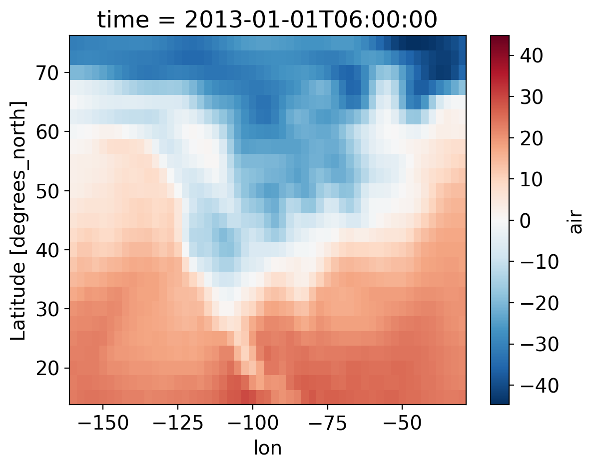
ds.air.isel(time=1).plot(x="lon")
<matplotlib.collections.QuadMesh at 0x7be0b40d0>
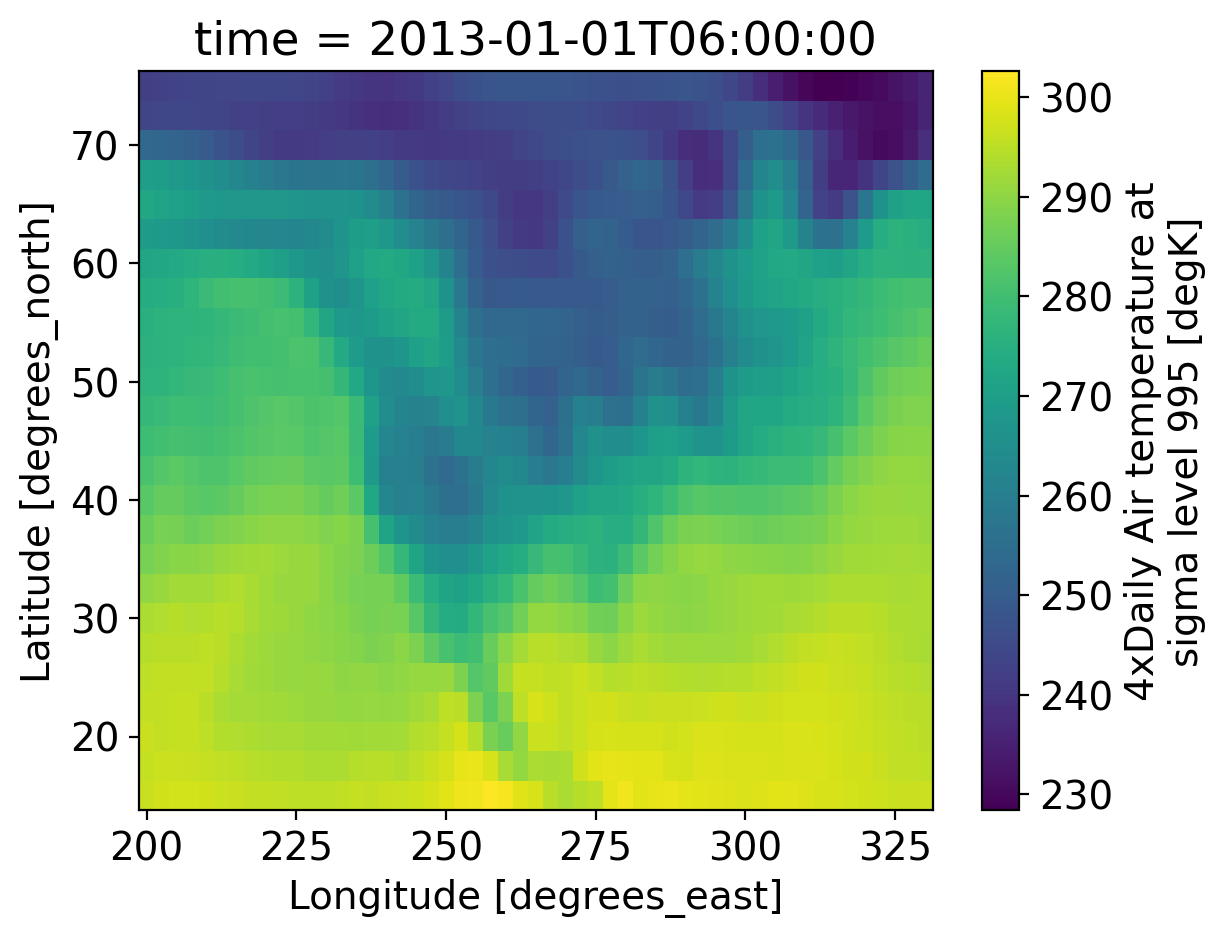
You would notice that the air temperature is in Kelvin. We can convert it to Celsius by removing 273.15 and changing the attributes units.
ds2=ds
ds2['air']=ds['air']-273.15
ds2['air']['units']='degC'
ds.air.isel(time=1).plot(x="lon")
<matplotlib.collections.QuadMesh at 0x7bd102370>
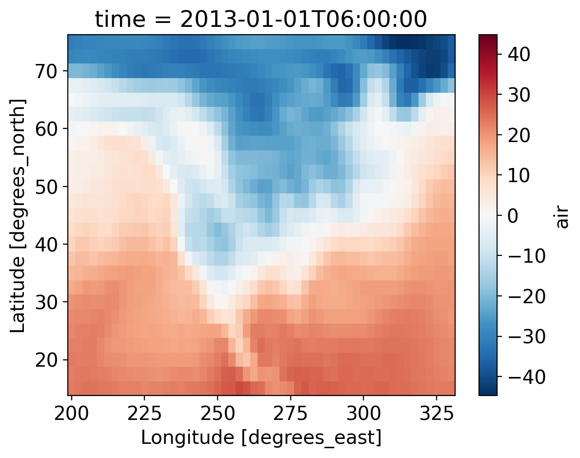
We also want to show the longitudes in the west direction by removing 360\(^\circ\).
ds2.coords["lon"]=ds2.coords["lon"]-360
ds.air.isel(time=1).plot(x="lon")
<matplotlib.collections.QuadMesh at 0x7be024760>
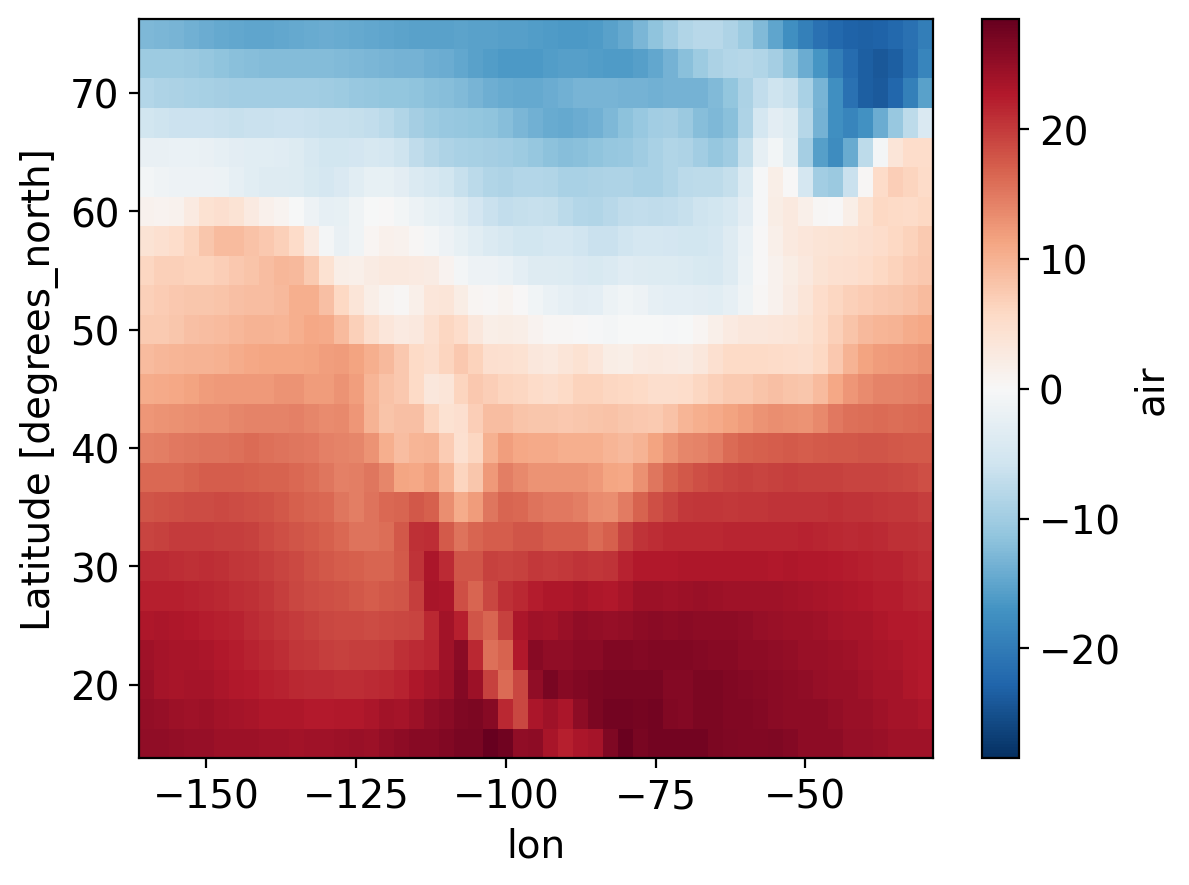
Show the mean temperature
ds2.air.mean("time").plot()
<matplotlib.collections.QuadMesh at 0x7be1fdf10>
ds2.sel(time="2013-05")
<xarray.Dataset>
Dimensions:  (lat: 25, time: 124, lon: 53)
Coordinates:
  * lat      (lat) float32 75.0 72.5 70.0 67.5 65.0 ... 25.0 22.5 20.0 17.5 15.0
  * time     (time) datetime64[ns] 2013-05-01 ... 2013-05-31T18:00:00
  * lon      (lon) float32 -160.0 -157.5 -155.0 -152.5 ... -35.0 -32.5 -30.0
Data variables:
    air      (time, lat, lon) float32 -13.95 -13.86 -14.05 ... 25.05 24.45 24.35
Attributes:
    Conventions:  COARDS
    title:        4x daily NMC reanalysis (1948)
    description:  Data is from NMC initialized reanalysis\n(4x/day).  These a...
    platform:     Model
references: http://www.esrl.noaa.gov/psd/data/gridded/data.ncep.reanaly...# demonstrate slicing
ds.sel(time=slice("2013-05", "2013-07"))
<xarray.Dataset>
Dimensions:  (lat: 25, time: 368, lon: 53)
Coordinates:
  * lat      (lat) float32 75.0 72.5 70.0 67.5 65.0 ... 25.0 22.5 20.0 17.5 15.0
  * time     (time) datetime64[ns] 2013-05-01 ... 2013-07-31T18:00:00
  * lon      (lon) float32 -160.0 -157.5 -155.0 -152.5 ... -35.0 -32.5 -30.0
Data variables:
    air      (time, lat, lon) float32 -13.95 -13.86 -14.05 ... 26.25 26.35 26.55
Attributes:
    Conventions:  COARDS
    title:        4x daily NMC reanalysis (1948)
    description:  Data is from NMC initialized reanalysis\n(4x/day).  These a...
    platform:     Model
references: http://www.esrl.noaa.gov/psd/data/gridded/data.ncep.reanaly...# "nearest indexing at multiple points"
ds.sel(lon=[240.125-360, 234-360], lat=[40.3, 50.3], method="nearest")
<xarray.Dataset>
Dimensions:  (lat: 2, time: 2920, lon: 2)
Coordinates:
  * lat      (lat) float32 40.0 50.0
  * time     (time) datetime64[ns] 2013-01-01 ... 2014-12-31T18:00:00
  * lon      (lon) float32 -120.0 -125.0
Data variables:
    air      (time, lat, lon) float32 -5.05 9.85 -7.65 ... 12.04 -16.36 -4.56
Attributes:
    Conventions:  COARDS
    title:        4x daily NMC reanalysis (1948)
    description:  Data is from NMC initialized reanalysis\n(4x/day).  These a...
    platform:     Model
references: http://www.esrl.noaa.gov/psd/data/gridded/data.ncep.reanaly...3.3 High level computation#
groupby : Bin data in to groups and reduce
resample : Groupby specialized for time axes. Either downsample or upsample your data.
rolling : Operate on rolling windows of your data e.g. running mean
coarsen : Downsample your data
weighted : Weight your data before reducing
# seasonal groups
ds.groupby("time.season")
# make a seasonal mean
seasonal_mean = ds.groupby("time.season").mean()
seasonal_mean = seasonal_mean.sel(season=["DJF", "MAM", "JJA", "SON"])
seasonal_mean
# resample to monthly frequency
ds.resample(time="M").mean()
# facet the seasonal_mean
seasonal_mean.air.plot(col="season")
We can save Xarrays in to NetCDF and Zarr files
# write to netCDF
%timeit ds.to_netcdf("my-example-dataset.nc")
!ls -lh my-example-dataset.nc
6.97 ms ± 326 µs per loop (mean ± std. dev. of 7 runs, 100 loops each)
-rw-r--r--@ 1 marinedenolle  staff    15M Oct  9 10:45 my-example-dataset.nc
%timeit ds.to_zarr(store="./my-example-dataset.zarr",mode="w")
!du -sh ./my-example-dataset.zarr
55.9 ms ± 1.89 ms per loop (mean ± std. dev. of 7 runs, 10 loops each)
 11M	./my-example-dataset.zarr
3.4 Student exercise#
Retrieve Air Temperature Data:
Use the air temperature data set and extract the time series at the latitude and longitude of Seattle.
Plot the Time Series:
Plot the time series of the air temperature data using matplotlib.
Fit a Sine Function:
Fit a sine function to the time series data using scipy.optimize.curve_fit.
# Latitude
l

# Longitude
# extract the air temperature data at these latitude and longitude
# extract the time series, print its data type, and convert it to numerical values
# plot the data with appropriate labels and legends
# import the curve_fit function from scipy.optimize
# define a function to take the time series data and fit it to a sinusoidal function
#
4. Pytorch Tensors#
This material is extracted from the Pytorch Package materials and from Dive into Deep Learning
The tensor class in Pytorch is similar to an ndarray in Numpy, with the added features that: 1) it has automatic differentiation and 2) it runs on CPUs and GPUs.
import torch
We can define a basic tensor that will be by default a 1-D array (vector) and run on the CPU
x = torch.arange(12, dtype=torch.float32)
x
Each value is refered to as an element. We can extract the length of the vector using the method numel() (a method is applied with ()) and its attribute shape is found by applyingshape
x.numel()
x.shape
We can reshape a tensor and flip dimensions
x.reshape(12,1).shape
x2=x.reshape(3,4)
x2.shape
We can create a random tensor
x3=torch.randn(3, 4)
We can apply element-wise operations on the tensor simply as methods. Here is an example by applying the function exp to all elements of the random tensor x3.
x3.exp()
We can manipulate 2 arrays of the same shape
x = torch.tensor([1.0, 2, 4, 8])
y = torch.tensor([2, 2, 2, 2])
x + y, x - y, x * y, x / y, x ** y
We can normalize the tensor with its L2 norm. Try below
x /=np.linalg.norm(x)
x
We can convert a numpy array to a Pytorch tensor
a=x.numpy()
print(type(a))
print(type(x))
Move an array from CPU to GPU by changing the device attribute
device = torch.device("cpu")
print(device)
Below, we are going to perform a regression to write a sine function as a function
import torch
import math


dtype = torch.float
device = torch.device("cpu")
# device = torch.device("cuda:0") # Uncomment this to run on GPU

# Create random input and output data
x = torch.linspace(-math.pi, math.pi, 2000, device=device, dtype=dtype)
y = torch.sin(x)

# Randomly initialize weights
a = torch.randn((), device=device, dtype=dtype)
b = torch.randn((), device=device, dtype=dtype)
c = torch.randn((), device=device, dtype=dtype)
d = torch.randn((), device=device, dtype=dtype)

learning_rate = 1e-6
for t in range(2000):
    # Forward pass: compute predicted y
    y_pred = a + b * x + c * x ** 2 + d * x ** 3

    # Compute and print loss
    loss = (y_pred - y).pow(2).sum().item()
    if t % 100 == 99:
        print(t, loss)

    # Backprop to compute gradients of a, b, c, d with respect to loss
    grad_y_pred = 2.0 * (y_pred - y)
    grad_a = grad_y_pred.sum()
    grad_b = (grad_y_pred * x).sum()
    grad_c = (grad_y_pred * x ** 2).sum()
    grad_d = (grad_y_pred * x ** 3).sum()

    # Update weights using gradient descent
    a -= learning_rate * grad_a
    b -= learning_rate * grad_b
    c -= learning_rate * grad_c
    d -= learning_rate * grad_d


print(f'Result: y = {a.item()} + {b.item()} x + {c.item()} x^2 + {d.item()} x^3')
5. Comparison of NumPy, Xarray, and PyTorch#
Feature/Use Case |
NumPy |
Xarray |
PyTorch |
|---|---|---|---|
Basic Array Manipulation |
Excellent |
Good |
Good |
Labeled Dimensions |
Limited |
Excellent |
Limited |
Multi-dimensional Data Support |
Excellent |
Excellent |
Excellent |
Deep Learning Integration |
Limited |
Limited |
Excellent |
GPU Acceleration |
None |
None |
Excellent |
Geoscientific Data (climate, etc.) |
Possible but requires effort |
Excellent |
Possible |
Choosing the Right Tool for the Task#
NumPy: Best for basic numerical operations and standard array manipulation.
Xarray: Ideal for labeled, multi-dimensional geoscientific datasets, particularly in climate modeling, remote sensing, and spatial data.
PyTorch: Best when applying machine learning or deep learning models to geoscientific data, especially when dealing with large datasets and requiring GPU acceleration.
Array Conversions#
Task:
Convert the xarray of air temperature into a 3D numpy and a 3D pytorch array
systematically print the dimensions
