Epipelargosy

Epipelargosy#

Wavering between the profit and the loss in this brief transit where the dreams cross…

-T.S.Eliot

Epipelargosy (επιπελαργοση)(noun)(neologism): A voyage through the epipelagic zone.

This chapter introduces physical and bio-optical data from a shallow profiler as pictured below. We will also look at data from a NOAA buoy installed about one kilometer away that tracks the surface sea state including waves and wind conditions.

To begin with the shallow profiler: Let’s review how observational data are collected. The profiler base or platform is anchored to the sea floor by cables. The platform is positively buoyant, ‘floating’ 200 meters below the ocean surface. Periodically cable is let out from the platform so that the instrument-bearing science pod (upper right in image) gradually ascends from the platform depth to a few meters below the surface, acquiring data as it rises. The science pod is then drawn back down. In this manner the instruments on the science pod profile the upper water column through a depth range of 10 to 200 meters. Typically there are nine such profiles per day.

Image('../img/shallowprofilerinsitu.png', width=400)

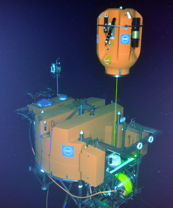
../_images/2e55b24d91a59b1d9df5701bf633a5b8567ad7d2070c3968aa0fe7ca6114ecde.png

Shallow Profiler: Platform and Science Pod photographed by an ROV; depth 200 meters. The orange sensor pod (the Science Pod or SCIP) is tethered to the rectangular platform (yellow cable). Multiple instruments are attached to the SCIP bearing one or more sensors. Sensors acquire data: Temperature, salinity, fluorescence and so on.

The shallow profiler platform resides at a site (i.e. a geographic location). Sites are connected together by means of undersea cables. The ensemble constitutes an enormous observing system called the Regional Cabled Array (RCA). The RCA is in turn one of several arrays that together comprise the Ocean Observatories Initiative.

Technical notes#

Code and data organization#

The code in this notebook uses a data dictionary to manage the large collection of sensors intrinsic to the RCA shallow profilers. This dictionary is elaborated at some length in the shallowprofiler_techical.ipynb notebook. In addition there are several native module files (file extension .py) that contain commonly used functions: See charts.py, data.py and shallowprofiler.py for example.

The `/osb` data path#

The data volume in use here exceeds the recommended limit for GitHub. Consequently we use a standard Linux mechanism to place the data outside the repository while making it appear functionally like it is inside. This mechanism is called a symbolic link.

The notebook dataloader.ipynb is run to build out a dataset from the Oregon Slope Base shallow profiler. The Oregon Slope Base site is abbreviated osb. The data should be placed in a local directory outside the repo, for example in /home/user/osb. A symbolic link is then created inside this repository that links or points to this external data directory. The Linux command to generate this link would be something like:

ln -s /home/user/osb /home/user/oceanography/books/chapters/data/rca/sensors/osb

This command should be customized to fit the file paths on your system.

Load profile metadata and build the data dictionary#

We now presume the osb data has been loaded and linked as described above.
The next step – cell below – is to build out a data dictionary d with keys corresponding to sensors: conductivity, temperature, pco2 etcetera. Sensor names are the dictionary keys. The dictionary values are five-tuples indexed \[0\], \[1\], \[2\], \[3\], \[4\]. These correspond to two XArray DataArrays, 2 float values, and one string respectively:

XArray DataArray: sensor data: Various units, coordinate/dimension = time
XArray DataArray: sensor depth: Meters, coordinate/dimension = time
float: Default charting lower limit for this sensor's data
float: Default charting upper limit for this sensor's data
string: Default chart color e.g. 'blue'

Note that if the time extent of the data is one month – say 30 days – a shallow profiler will generate about \(9 \times 30 = 270\) profiles. Selecting out time blocks that correspond to these profiles is done using the profile metadata, contained in a pandas Dataframe called profiles.

We interrupt this broadcast#

import shallowprofiler as sp
from data import *
from charts import *
from os import path
from time import time

Jupyter Notebook running Python 3

# Loads data / depth from local files > d{}. See the chapter 'dataloader' to pre-stage these local files. 
#   Each sensor has an associated key so d[key] is a 5-tuple (DA-sensor, DA-depth, lo, hi, color).

profiles = ReadProfileMetadata()                   # Times associated with profile stages, 1 year
# print(profiles)
print(type(profiles['a0t'][0]))

<class 'pandas._libs.tslibs.timestamps.Timestamp'>

data_file_root_path   = './data/rca/sensors'
sitestring            = 'osb'
monthstring           = 'jan'               
yearstring            = '2022'
fTemp     = AssembleShallowProfilerDataFilename(data_file_root_path, sitestring, "temp", monthstring, yearstring)
fSalinity = AssembleShallowProfilerDataFilename(data_file_root_path, sitestring, "salinity", monthstring, yearstring)
print(fTemp, fSalinity)

./data/rca/sensors/osb/temp_jan_2022.nc ./data/rca/sensors/osb/salinity_jan_2022.nc

Tds = xr.open_dataset(fTemp)
Sds = xr.open_dataset(fSalinity)

---------------------------------------------------------------------------
KeyError                                  Traceback (most recent call last)
File ~/micromamba/envs/geosmart-template/lib/python3.12/site-packages/xarray/backends/file_manager.py:211, in CachingFileManager._acquire_with_cache_info(self, needs_lock)
    210 try:
--> 211     file = self._cache[self._key]
    212 except KeyError:

File ~/micromamba/envs/geosmart-template/lib/python3.12/site-packages/xarray/backends/lru_cache.py:56, in LRUCache.__getitem__(self, key)
     55 with self._lock:
---> 56     value = self._cache[key]
     57     self._cache.move_to_end(key)

KeyError: [<class 'netCDF4._netCDF4.Dataset'>, ('/home/runner/work/oceanography/oceanography/book/chapters/data/rca/sensors/osb/temp_jan_2022.nc',), 'r', (('clobber', True), ('diskless', False), ('format', 'NETCDF4'), ('persist', False)), '235fba75-d5cc-4d2a-8c0c-4c7d1d89c7b5']

During handling of the above exception, another exception occurred:

FileNotFoundError                         Traceback (most recent call last)
Cell In[6], line 1
----> 1 Tds = xr.open_dataset(fTemp)
      2 Sds = xr.open_dataset(fSalinity)

File ~/micromamba/envs/geosmart-template/lib/python3.12/site-packages/xarray/backends/api.py:686, in open_dataset(filename_or_obj, engine, chunks, cache, decode_cf, mask_and_scale, decode_times, decode_timedelta, use_cftime, concat_characters, decode_coords, drop_variables, inline_array, chunked_array_type, from_array_kwargs, backend_kwargs, **kwargs)
    674 decoders = _resolve_decoders_kwargs(
    675     decode_cf,
    676     open_backend_dataset_parameters=backend.open_dataset_parameters,
   (...)    682     decode_coords=decode_coords,
    683 )
    685 overwrite_encoded_chunks = kwargs.pop("overwrite_encoded_chunks", None)
--> 686 backend_ds = backend.open_dataset(
    687     filename_or_obj,
    688     drop_variables=drop_variables,
    689     **decoders,
    690     **kwargs,
    691 )
    692 ds = _dataset_from_backend_dataset(
    693     backend_ds,
    694     filename_or_obj,
   (...)    704     **kwargs,
    705 )
    706 return ds

File ~/micromamba/envs/geosmart-template/lib/python3.12/site-packages/xarray/backends/netCDF4_.py:666, in NetCDF4BackendEntrypoint.open_dataset(self, filename_or_obj, mask_and_scale, decode_times, concat_characters, decode_coords, drop_variables, use_cftime, decode_timedelta, group, mode, format, clobber, diskless, persist, auto_complex, lock, autoclose)
    644 def open_dataset(
    645     self,
    646     filename_or_obj: str | os.PathLike[Any] | ReadBuffer | AbstractDataStore,
   (...)    663     autoclose=False,
    664 ) -> Dataset:
    665     filename_or_obj = _normalize_path(filename_or_obj)
--> 666     store = NetCDF4DataStore.open(
    667         filename_or_obj,
    668         mode=mode,
    669         format=format,
    670         group=group,
    671         clobber=clobber,
    672         diskless=diskless,
    673         persist=persist,
    674         auto_complex=auto_complex,
    675         lock=lock,
    676         autoclose=autoclose,
    677     )
    679     store_entrypoint = StoreBackendEntrypoint()
    680     with close_on_error(store):

File ~/micromamba/envs/geosmart-template/lib/python3.12/site-packages/xarray/backends/netCDF4_.py:452, in NetCDF4DataStore.open(cls, filename, mode, format, group, clobber, diskless, persist, auto_complex, lock, lock_maker, autoclose)
    448     kwargs["auto_complex"] = auto_complex
    449 manager = CachingFileManager(
    450     netCDF4.Dataset, filename, mode=mode, kwargs=kwargs
    451 )
--> 452 return cls(manager, group=group, mode=mode, lock=lock, autoclose=autoclose)

File ~/micromamba/envs/geosmart-template/lib/python3.12/site-packages/xarray/backends/netCDF4_.py:393, in NetCDF4DataStore.__init__(self, manager, group, mode, lock, autoclose)
    391 self._group = group
    392 self._mode = mode
--> 393 self.format = self.ds.data_model
    394 self._filename = self.ds.filepath()
    395 self.is_remote = is_remote_uri(self._filename)

File ~/micromamba/envs/geosmart-template/lib/python3.12/site-packages/xarray/backends/netCDF4_.py:461, in NetCDF4DataStore.ds(self)
    459 @property
    460 def ds(self):
--> 461     return self._acquire()

File ~/micromamba/envs/geosmart-template/lib/python3.12/site-packages/xarray/backends/netCDF4_.py:455, in NetCDF4DataStore._acquire(self, needs_lock)
    454 def _acquire(self, needs_lock=True):
--> 455     with self._manager.acquire_context(needs_lock) as root:
    456         ds = _nc4_require_group(root, self._group, self._mode)
    457     return ds

File ~/micromamba/envs/geosmart-template/lib/python3.12/contextlib.py:137, in _GeneratorContextManager.__enter__(self)
    135 del self.args, self.kwds, self.func
    136 try:
--> 137     return next(self.gen)
    138 except StopIteration:
    139     raise RuntimeError("generator didn't yield") from None

File ~/micromamba/envs/geosmart-template/lib/python3.12/site-packages/xarray/backends/file_manager.py:199, in CachingFileManager.acquire_context(self, needs_lock)
    196 @contextlib.contextmanager
    197 def acquire_context(self, needs_lock=True):
    198     """Context manager for acquiring a file."""
--> 199     file, cached = self._acquire_with_cache_info(needs_lock)
    200     try:
    201         yield file

File ~/micromamba/envs/geosmart-template/lib/python3.12/site-packages/xarray/backends/file_manager.py:217, in CachingFileManager._acquire_with_cache_info(self, needs_lock)
    215     kwargs = kwargs.copy()
    216     kwargs["mode"] = self._mode
--> 217 file = self._opener(*self._args, **kwargs)
    218 if self._mode == "w":
    219     # ensure file doesn't get overridden when opened again
    220     self._mode = "a"

File src/netCDF4/_netCDF4.pyx:2521, in netCDF4._netCDF4.Dataset.__init__()

File src/netCDF4/_netCDF4.pyx:2158, in netCDF4._netCDF4._ensure_nc_success()

FileNotFoundError: [Errno 2] No such file or directory: '/home/runner/work/oceanography/oceanography/book/chapters/data/rca/sensors/osb/temp_jan_2022.nc'

print(Tds)
print(Sds)

<xarray.Dataset>
Dimensions:  (time: 2678084)
Coordinates:
  * time     (time) datetime64[ns] 2022-01-01T00:00:00.097717760 ... 2022-01-...
Data variables:
    depth    (time) float64 ...
    temp     (time) float64 ...
<xarray.Dataset>
Dimensions:   (time: 2678084)
Coordinates:
  * time      (time) datetime64[ns] 2022-01-01T00:00:00.097717760 ... 2022-01...
Data variables:
    salinity  (time) float64 ...
    depth     (time) float64 ...

xr.open_dataset(fTemp).to_dataframe().to_csv('temp.csv')

df = xr.open_dataset(fSalinity).to_dataframe()
print(df.columns)

Index(['salinity', 'depth'], dtype='object')

df
# order is time, salinity, depth

	salinity	depth
time
2022-01-01 00:00:00.097717760	33.939419	192.457638
2022-01-01 00:00:01.097620992	33.939160	192.461935
2022-01-01 00:00:02.097106944	33.939271	192.467264
2022-01-01 00:00:03.097217536	33.939203	192.470428
2022-01-01 00:00:04.097119744	33.939189	192.475723
...	...	...
2022-01-31 23:59:55.066199552	33.912604	193.535232
2022-01-31 23:59:56.065684480	33.912751	193.533133
2022-01-31 23:59:57.066420736	33.912380	193.532067
2022-01-31 23:59:58.065696768	33.912450	193.532067
2022-01-31 23:59:59.066327552	33.912525	193.534199

2678084 rows × 2 columns

print(df.columns)

Index(['depth', 'salinity'], dtype='object')

df = df[['depth', 'salinity']]
print(df)

                                    depth   salinity
time                                                
2022-01-01 00:00:00.097717760  192.457638  33.939419
2022-01-01 00:00:01.097620992  192.461935  33.939160
2022-01-01 00:00:02.097106944  192.467264  33.939271
2022-01-01 00:00:03.097217536  192.470428  33.939203
2022-01-01 00:00:04.097119744  192.475723  33.939189
...                                   ...        ...
2022-01-31 23:59:55.066199552  193.535232  33.912604
2022-01-31 23:59:56.065684480  193.533133  33.912751
2022-01-31 23:59:57.066420736  193.532067  33.912380
2022-01-31 23:59:58.065696768  193.532067  33.912450
2022-01-31 23:59:59.066327552  193.534199  33.912525

[2678084 rows x 2 columns]

df.to_csv('salinity.csv')

d = {}                # empty dictionary: to populate with 5-tuples, default time range January 2022,
                      # defult site Oregon Slope Base

data_file_root_path   = './data/rca/sensors'
sitestring            = 'osb'
monthstring           = 'jan'               
yearstring            = '2022'

for sensor in sensors:   # sensors[] is a list of 2-element lists, each list = [sensor_str, instrument_str]
    f = AssembleShallowProfilerDataFilename(data_file_root_path, sitestring, sensor[0], monthstring, yearstring)
    if path.isfile(f): d[sensor[0]] = GetSensorTuple(sensor[0], f)    # creates d[sensor-key]
    # as a quick check on data validity: use d['temperature'].z.plot()

profile_list = [0]
d.keys()                    # indicates which sensors loaded properly: 'conductivity' etcetera

# `sensors` is a list of lists, each ['<sensor-name>', '<instrument-name>'].
# sensors

For a month like January 2022 there are 2678400 seconds.

d[] is a dictionary of tuples so d['temp'] has indices 0, 1 (both Data Arrays), 2, 3, 4. The latter are respectively real, real, str (a chart color). The real numbers are low and high values for the sensor. The five-tuple is designed to make it easy to produce charts comparing two sensor profiles.

sensortypes = ['salinity', 'temp']
for s in sensortypes:
    print(type(d[s][1]))
    print(d[s][2])
    print(d[s][3])
    print(d[s][4])

T=d['temp'][0]
T
Z=d['temp'][1]
Z

Ax, Ay = A.sel(time=slice(tA0,  tA1)), Az.sel(time=slice(tA0, tA1))

d['temp'][0]

type(d)

ChartSensor(profiles, [7, 11], [0], d['temp'][0], d['temp'][1], "temp", "red", 'ascent', 10, 10, z0=-200., z1=0.)

toc = time()
fig,axs = ChartTwoSensors(profiles, [ranges['temp'], ranges['salinity']], profile_list, 
                          d['temp'][0],     -d['temp'][1],     'Temperature', colors['temp'],     'ascent',
                          d['salinity'][0], -d['salinity'][1], 'Salinity',    colors['salinity'], 'ascent', 6, 6)
print(time() - toc, 'seconds\n\n\n')

Interpretation#

The upper 70m is a homogeneous mixed layer. The transitional section below this (particularly in terms of salinity) from 70m to 95m represents a sharp change in temperature and salinity. This is the pycnocline, a boundary separating the mixed layer from the lower ocean. From 95m down to the lowest observed depth of 195m we have water that is colder, more saline, and more dense. The cold temperature excursion in the data in the 70–90m depth range is an anomalous departure from a monotonic gradient.

# density and pressure
fig,axs = ChartTwoSensors(profiles, [ranges['density'], ranges['conductivity']], profile_list, 
                          d['density'][0],      -d['density'][1],      'Density',      colors['density'],    'ascent',
                          d['conductivity'][0], -d['conductivity'][1], 'Conductivity', 'blue', 'ascent', 6, 6)

Interpretation: …hmmmm… compared to the one prior: It seems like conductivity and salinity are not ‘pretty much the same thing’…

# dissolved oxygen and chlorophyll-a
fig,axs = ChartTwoSensors(profiles, [ranges['do'], ranges['chlora']], profile_list, 
                          d['do'][0],     -d['do'][1], 'Dissolved Oxygen', colors['do'],    'ascent',
                          d['chlora'][0], -d['chlora'][1],    'Chlorophyll-A',  colors['chlora'], 'ascent', 6, 6)

# fdom and backscatter
fig,axs = ChartTwoSensors(profiles, [ranges['fdom'], ranges['backscatter']], profile_list, 
                          d['fdom'][0],         -d['fdom'][1],        'FDOM', colors['do'], 'ascent',
                          d['backscatter'][0],  -d['backscatter'][1], 'Backscatter', colors['chlora'], 'ascent', 6, 6)

# pH and pCO2
# These sensors are recording only on midnight and noon *descents*. The first of these 0n
# January 1 2022 is profile 3, not profile 0, hence the third argument is [3], the first 
# first midnight profile of January. Next would be profiel 8, the subsequent noon. 
fig,axs = ChartTwoSensors(profiles, [ranges['ph'], ranges['pco2']], [3],
                          d['ph'][0],    -d['ph'][1], 'pH', colors['ph'], 'descent',
                          d['pco2'][0],  -d['pco2'][1], 'pCO2', colors['pco2'], 'descent', 6, 6)

# Spectral irradiance is not currently in place
if False:
    fig,axs = ChartTwoSensors(profiles, [ranges['spkir412nm'], ranges['spkir555nm']], [8],
                              d['spkir412nm'][0], d['spkir412nm'][1], '412nm', colors['spkir412nm'], 'ascent',
                              d['spkir555nm'][0], d['spkir555nm'][1], '555nm', colors['spkir555nm'], 'ascent', 6, 6)

if False:
    fig,axs = ChartTwoSensors(profiles, [ranges['par'], ranges['spkir620nm']], [8, 80],
                              d['par'][0], d['par'][1], 'PAR', colors['par'], 'ascent',
                              d['spkir620nm'][0], d['spkir620nm'][1], 'spkir620nm spkir', 
                              colors['spkir620nm'], 'ascent', 6, 6)

# Nitrate and pH (midnight: ascent for nitrate, descent for pH)
fig,axs = ChartTwoSensors(profiles, [ranges['nitrate'], ranges['ph']], [3],     # (then 8, 12, 17)
                          d['nitrate'][0], -d['nitrate'][1], 'nitrate', colors['nitrate'], 'ascent',
                          d['ph'][0], -d['ph'][1], 'pH', colors['ph'], 'descent', 6, 6)

# Current velocity 'east' and 'north'
fig,axs = ChartTwoSensors(profiles, [ranges['east'], ranges['north']], [0],
                          d['east'][0], -d['east'][1], 'east velocity', colors['east'], 'ascent',
                          d['north'][0], -d['north'][1], 'north velocity', colors['north'], 'ascent', 6, 4)

A next type of visualization: bundle charts#

The ‘depth-signal’ charts above illustrate epipelagic snapshots in terms of single profiles. A next logical step is to create ‘bundle charts’ from consecutive profiles for a given sensor. This introduces a sense of variability across a longer time interval. Again we note that nine consecutive profiles correspond to a single day.

if False: ShowStaticBundles(d, profiles)   # broken

def BundleChart(profiles, date0, date1, time0, time1, wid, hgt, data, title):
    '''
    Create a bundle chart: Multiple profiles showing sensor/depth in ensemble.
        date0   start / end of time range: date only, range is inclusive [date0, date1]
        date1
        time0   start / end time range for each day
        time1       (this scheme permits selecting midnight or noon)
        wid     figure size
        hgt
        data    a value from the data dictionary (5-tuple: includes range and color)
        title   chart title
    '''

BundleChart(profiles, dt64('2022-01-01'), dt64('2022-02-01'), td64(0, 'h'), td64(24, 'h'), 8, 6,  'Dissolved Oxygen')

def LocalGenerateTimeWindowIndices(profiles, dt0, dt1):
    '''
    In UTC: Passed a time window via two bounding datetimes. Return a list of 
    profile indices for profiles that begin ascent within this time box. These 
    indices are rows in the profiles DataFrame.
    '''
    pidcs = []
    for i in range(len(profiles)):
        a0 = profiles["a0t"][i]
        if a0 >= dt0 and a0 <= dt1: pidcs.append(i)
    return pidcs


def LocalBundleChart(profiles, dt0, dt1, wid, hgt, data, depth, lo, hi, title, color):
    pidcs = LocalGenerateTimeWindowIndices(profiles, dt0, dt1)
    if len(pidcs) < 1: 
        print('LocalBundleChart(): Zero profile hits')
        return False
    fig, ax = plt.subplots(figsize=(wid, hgt), tight_layout=True)
    for i in range(len(pidcs)):
        ta0, ta1 = profiles["a0t"][pidcs[i]], profiles["a1t"][pidcs[i]]
        ax.plot(data.sel(time=slice(ta0,  ta1)), depth.sel(time=slice(ta0, ta1)), ms = 4., color=color)
    ax.set(title = title)
    ax.set(xlim = (lo, hi), ylim = (-200, 0))
    return ax

bundle_start_time, bundle_end_time = dt64('2022-01-01T00:00:00'), dt64('2022-01-04T00:00:00')
LocalBundleChart(profiles, bundle_start_time, bundle_end_time, 
                 8, 8, d['do'][0], -d['do'][1], d['do'][2], d['do'][3], 'Dissolved Oxygen: OSB, 3 days', d['do'][4])

bundle_start_time, bundle_end_time = dt64('2022-01-01T00:00:00'), dt64('2022-02-01T00:00:00')
LocalBundleChart(profiles, bundle_start_time, bundle_end_time, 
                 8, 8, d['do'][0], -d['do'][1], d['do'][2], d['do'][3], 'Dissolved Oxygen', d['do'][4])

Interpretation#

The three-day time interval implies at most 27 profiles. Some might be missing. The low profile depth is fairly consistently around 195 meters. The upper depth shows more variability, 10 to 30 meters.

The mixed layer depth (transition to pycnocline) varies in depth from 50 to 70 meters. Mixed layer depth is influenced by surface winds driving wave action and hence mixing.

There are anomalies in the month-long dataset: Dissolved oxygen excursions below the main ‘bundle’. In particular four ‘low oxygen’ profiles originate in the pycnocline and extend down to the platform depth at 190 meters. To verify that these profiles are consecutive we need a convenient scrolling interface; which we now introduce by means of an interactive ‘widget’.

from ipywidgets import interact, widgets
from traitlets import dlink

def BundleInteract(sensor_key, time_index, bundle_size):
    '''
    Consider a time range that includes many (e.g. 279) consecutive profiles. This function plots sensor data
    within the time range. Choose the sensor using a dropdown. Choose the first profile using the start slider.
    Choose the number of consecutive profiles to chart using the bundle slider. 
    Details
      - There is no support at this time for selecting midnight or noon profiles exclusively
          - nitrate, ph and pco2 bundle charts will be correspondingly sparse
      - There is a little bit of intelligence built in to the selection of ascent or descent
          - most sensors measure on ascent or ascent + descent. pco2 and ph are descent only
          - ph and pco2 still have a charting bug "last-to-first line" clutter: For some reason
            the first profile value is the last value from the prior profile. There is a hack in
            place ("i0") to deal with this.
      - All available profiles are first plotted in light grey
          - This tacitly assumes a month or less time interval for the current full dataset
    '''
    
    
    (phase0, phase1, i0) = ('a0t', 'a1t', 0) if not (sensor_key == 'ph' or sensor_key == 'pco2') else ('d0t', 'd1t', 1)
    x    = d[sensor_key][0]
    z    = d[sensor_key][1]
    xlo = d[sensor_key][2]
    xhi = d[sensor_key][3]
    xtitle = sensor_names[sensor_key]
    xcolor = d[sensor_key][4]

    # This configuration code block is hardcoded to work with Jan 2022
    date0, date1   = dt64('2022-01-01T00:00:00'), dt64('2022-02-01T00:00:00')
    wid, hgt       = 9, 6
    x0, x1, z0, z1 = xlo, xhi, -200, 0
    title          = xtitle
    color          = xcolor
    pidcs          = LocalGenerateTimeWindowIndices(profiles, date0, date1)    # !!!!! either midn or noon, not both
    nProfiles      = len(pidcs)
    
    fig, ax = plt.subplots(figsize=(wid, hgt), tight_layout=True)
    
    # insert code: light grey full history
    iProf0 = 0
    iProf1 = nProfiles
    for i in range(iProf0, iProf1):
        pIdx = pidcs[i]
        ta0, ta1 = profiles[phase0][pIdx], profiles[phase1][pIdx]
        xi, zi = x.sel(time=slice(ta0,  ta1)), -z.sel(time=slice(ta0, ta1))
        ax.plot(xi[i0:], zi[i0:], ms = 4., color = 'xkcd:light grey')    
    
    # resume normal code
    iProf0 = time_index if time_index < nProfiles else nProfiles
    iProf1 = iProf0 + bundle_size if iProf0 + bundle_size < nProfiles else nProfiles
    for i in range(iProf0, iProf1):
        pIdx = pidcs[i]
        ta0, ta1 = profiles[phase0][pIdx], profiles[phase1][pIdx]
        xi, zi = x.sel(time=slice(ta0,  ta1)), -z.sel(time=slice(ta0, ta1))
        ax.plot(xi[i0:], zi[i0:], ms = 4., color=color, mfc=color)
    ax.set(title = title)
    ax.set(xlim = (x0, x1), ylim = (z0, z1))

    # Add text indicating the current time range of the profile bundle
    # tString = str(p["ascent_start"][pIdcs[iProf0]])
    # if iProf1 - iProf0 > 1: tString += '\n ...through... \n' + str(p["ascent_start"][pIdcs[iProf1-1]])
    # ax.text(px, py, tString)
    
    plt.show()
    return

def Interactor(continuous_update = False):
    '''Set up three bundle-interactive charts, vertically. Independent sliders for choice of 
    sensor, starting profile by index, and number of profiles in bundle. (90 profiles is about
    ten days.) A fast machine can have cu = True to give a slider-responsive animation. Make
    it False to avoid jerky 'takes forever' animation on less powerful machines.
    '''
    style = {'description_width': 'initial'}
    
    # data dictionary d{} keys:
    optionsList = ['temp', 'salinity', 'density', 'conductivity', 'do', 'chlora', 'fdom', 'bb', 'pco2', \
                   'ph', 'par', 'nitrate', 'east', 'north', 'up']

    interact(BundleInteract, \
                             sensor_key = widgets.Dropdown(options=optionsList,  value=optionsList[0], description='sensor'), \
                             time_index = widgets.IntSlider(min=0, max=270, step=1, value=160,                    \
                                                            layout=widgets.Layout(width='35%'),                   \
                                                            continuous_update=False, description='bundle start',  \
                                                            style=style),
                             bundle_size = widgets.IntSlider(min=1, max=90, step=1, value=20,                     \
                                                            layout=widgets.Layout(width='35%'),                   \
                                                            continuous_update=False, description='bundle width',  \
                                                            style=style))

    return

Interactor(False)

Interpretation#

Selecting dissolved oxygen (do) with start = 0, width = 90 shows two anomalies, both low oxygen levels. The full bundle is shown in light grey in the background for context. Narrowing in we get start = 59 and width = 4 showing four consecutive anomalous profiles. The anomaly extends as far down as the profiler platform at ~195 meters.

The bundle width slider can be maximized to reinforce the typical (bundle-based) profile distribution in relation to the second anomaly.

Incidentally other anomalies are also apparent, for example a single outlier in profile 211.

Temperature coincidence: An obvious next thought is to check for coincidence: This dissolved oxygen anomaly with other sensors. Beginning with temperature: During the anomaly the mixed layer is apparently very small (30 meters) with a relatively cold upper water column temperature. Sub-pycnocline temperatures are in contrast comparatively warm. The pycnocline itself is very constricted and features temperature inversions.

Salinity coincidence: The anomaly is again present, with a shallow fixed layer and comparatively high salinity throughout the profiler depth range.

Density coincidence: Sharp increase through the pycnocline, anomalously high.

Other coincidences: pH, pCO2, nitrate, chlorophyll: All anomalous, respectively low, high, high, low.

Interactor(False)
Interactor(False)
Interactor(False)

ZuluToLocal = td64(8, 'h')
for i in range(4): print(profiles['a0t'][59+i]-ZuluToLocal)
print('\n\nZulu\n')
for i in range(4): print(profiles['a0t'][59+i]-ZuluToLocal)

Summary: The OSB shallow profiler observed a mass of acidic, nutrient rich water with depleted oxygen and elevated carbon dioxide on January 7 2022. The episode lasted ten hours.

Questions about the sea state

What was the current before / during / after this anomaly?
Was the onset sharp or gradual? Decay to typical sharp or gradual?
What was the windspeed? Wave height?

The NOAA National Data Buoy Center (NDBC) has historical data available for download. This website is the search interface. Stations 46098 and 46050 are closest to the Oregon Slope Base observing site: Respective distances are 1 km and 46 km. Datasets are downloadable as text files (space delimiter). No-data values typically have nines in them, as 999 or 99.00 or 999.0. Observations are at 10 minute intervals.

Historical buoy data: Metadata#

The first two rows of a data file are column headers: Type and units. An interpretive key may be found here. For the two stations of interest, 46098 and 46050, year = 2022, we have these column headers:

YY  MM DD hh mm     Time down to minutes: UTC not local
WDIR WSPD GST       Wind speed, direction and gusts; direction is degrees clockwise from true north
WVHT                Wave height, meters
DPD   APD           Dominant and Average wave period
MWD                 Mean wave direction (direction from which; deg CW from TN as above)
PRES                Sea surface atmospheric pressure (hPa, hectoPascale or equiv. millibars)
ATMP                Air temperature (deg C)
WTMP                Surface water temperature (deg C)
DEWP                Dewpoint (deg C)
VIS                 Visibility (mi)
TIDE                Tide (ft)

Locations, proximity#

Oregon Slope Base:  44.37415 N      124.95648 W
Buoy 46050:         44.669   N      124.546   W       Distance to OSB: 46km
Buoy 46098:         44.378   N      124.947   W       Distance to OSB:  1km

# This cell calculates distances from NDBC buoys to the OSB shallow profiler

from math import cos, pi, sqrt

loc_osb_lat, loc_osb_lon               = 44.37415, -124.95648
loc_buoy_46050_lat, loc_buoy_46050_lon = 44.669,   -124.546
loc_buoy_46098_lat, loc_buoy_46098_lon = 44.378,   -124.947

earth_r   = 6378000
earth_c   = earth_r * 2 * pi
deg_lat_m = earth_c / 360

print('one degree of latitude approximately', round(deg_lat_m, 1), 'meters')

meanlat    = (1/3)*(loc_osb_lat + loc_buoy_46050_lat + loc_buoy_46098_lat)
dtr        = pi/180
lon_stride = deg_lat_m * cos(meanlat*dtr)

print('At this latitude one degree of longitude is', round(lon_stride, 1), 'meters')

dlat = loc_osb_lat - loc_buoy_46050_lat
dlon = loc_osb_lon - loc_buoy_46050_lon
d_osb_46050 = sqrt((dlat*deg_lat_m)**2 + (dlon*lon_stride)**2)

dlat = loc_osb_lat - loc_buoy_46098_lat
dlon = loc_osb_lon - loc_buoy_46098_lon
d_osb_46098 = sqrt((dlat*deg_lat_m)**2 + (dlon*lon_stride)**2)

print('Distance OSB to buoy 46050:', round(d_osb_46050, 1), 'm')
print('Distance OSB to buoy 46098:', round(d_osb_46098, 1), 'm')

# This cell reads in the 46098 (proximal) data to a pandas DataFrame
ndbc_root_path     = './data/noaa/ndbc/'
buoy_id            = '46098'
year               = '2022'
ndbc_filename      = 'station_' + buoy_id + '_year_' + year + '.txt'
ndbc_path          = ndbc_root_path + ndbc_filename

# This cell can take a few minutes to run. It loads and tidies up the NDBC data from
#   a site 1km from the OSB shallow profiler location.
#
# def ReadNDBCMetadata(fnm = './data/noaa/ndbc/station_46098_year_2022.txt'):
#     """
#     See comment above on file format.
#     The default input buoy is 800 meters from the Oregon Slope Base (OSB) site. Default year is 2022.
#     """
df = pd.read_csv('./data/noaa/ndbc/station_46098_year_2022.txt', sep='\s+', header = 0)
df = df.drop([0])        # the second row of text is units for each column
# df
# df['Zulu'] = pd.to_datetime( )
# df['Zulu'] = pd.to_datetime(df['#YY'] + '-' + str(df['MM']) + '-' + str(df['DD']))
# df.dtypes gives all 'object'
# print(df['#YY'][17]) etcetera for MM DD hh mm

# timestamp = dt64(df['#YY'][1400] + '-' + df['MM'][1400] + '-' + df['DD'][1400] + ' ' + df['hh'][1400] + ':' + df['mm'][1400])
# print(timestamp)
# df['Zulu'] = pd.to_datetime(str(df['#YY']) + '-' + str(df['MM']) + '-' + str(df['DD']) + ' ' + str(df['hh']) + ':' + str(df['mm']))

df['Zulu'] = pd.to_datetime(df['#YY'])
for i in range(1, len(df)+1):
    c_yr = str(df['#YY'][i])
    c_mo = str(df['MM'][i])
    c_dy = str(df['DD'][i])
    c_hr = str(df['hh'][i])
    c_mn = str(df['mm'][i])      # eschewing fixes like: if len(c_mo) == 1: c_mo = '0' + c_mo
    df['Zulu'][i] = pd.to_datetime(c_yr + '-' + c_mo + '-' + c_dy + ' ' + c_hr + ':' + c_mn)

df = df.drop(columns=['#YY', 'MM', 'DD', 'hh', 'mm'])

df = df.astype({'WDIR': 'float'})
df = df.astype({'WSPD': 'float'})
df = df.astype({'GST': 'float'})
df = df.astype({'WVHT': 'float'})
df = df.astype({'DPD': 'float'})
df = df.astype({'APD': 'float'})
df = df.astype({'MWD': 'float'})
df = df.astype({'PRES': 'float'})
df = df.astype({'ATMP': 'float'})
df = df.astype({'WTMP': 'float'})
df = df.astype({'DEWP': 'float'})
df = df.astype({'VIS': 'float'})
df = df.astype({'TIDE': 'float'})             # to this point: df still contains 99 and 999 for "no data"
                                              #   so we take a moment to replace those with np.NaN.
dfNaN = df.replace([99, 999], np.NaN)         # Post-NaN-sub this fails: dfNaN['WVHT'][1:4459].plot()
dfNaN                                         # Visual inspection of the cleaned up DataFrame

# Artifact: Scatter plot
# fig,ax = plt.subplots(figsize=(8,8))
# ax.scatter(dfNaN['Zulu'][1:4459], dfNaN['WVHT'][1:4459], s=4, c='r')
# , ds.z, marker='.', ms=11., color='k', mfc='r', linewidth='.0001')
# ax.set(ylim = (0., 10.), title='OSB site wave height (meters) Jan 2022', ylabel='WVHT (m)', xlabel='Date')
# ax.set(xticks=[dt64('2022-01-01'), dt64('2022-01-15T12:00'), dt64('2022-02-01')])

wdir_time = dfNaN['Zulu'][1:4459]; wdir_data = dfNaN['WDIR'][1:4459]; wdir_mask = np.isfinite(wdir_data)
wvht_time = dfNaN['Zulu'][1:4459]; wvht_data = dfNaN['WVHT'][1:4459]; wvht_mask = np.isfinite(wvht_data)
wspd_time = dfNaN['Zulu'][1:4459]; wspd_data = dfNaN['WSPD'][1:4459]; wspd_mask = np.isfinite(wspd_data)
wtmp_time = dfNaN['Zulu'][1:4459]; wtmp_data = dfNaN['WTMP'][1:4459]; wtmp_mask = np.isfinite(wtmp_data)

fig,ax = plt.subplots(figsize=(12,6))
ax.plot(wvht_time[wvht_mask], wvht_data[wvht_mask], linestyle='-', marker='.', ms=3, color='red', mec='black')
ax.plot(profiles['a0t'][59], 5.8, linestyle='-', marker='.', color='blue')
ax.set(ylim = (0., 10.), title='OSB site wave height (meters) Jan 2022', ylabel='WVHT (m)', xlabel='Date')
ax.set(xticks=[dt64('2022-01-01'), dt64('2022-01-15T12:00'), dt64('2022-02-01')])

fig,ax = plt.subplots(figsize=(12,6))
twinx = ax.twinx()
ax.plot(wspd_time[wspd_mask], wspd_data[wspd_mask], linestyle='-', marker='.', ms=3, color='black', mec='blue')
ax.plot(profiles['a0t'][59], 5.8, linestyle='-', marker='.', color='blue')
ax.set(ylim = (0., 22.), title='OSB site wind speed (meters / second) Jan 2022', ylabel='WSPD (m/s)', xlabel='Date')
ax.set(xticks=[dt64('2022-01-01'), dt64('2022-01-15T12:00'), dt64('2022-02-01')])

twinx.plot(wvht_time[wvht_mask], wvht_data[wvht_mask], linestyle='-', marker='.', ms=3, color='red', mec='black')
twinx.set(ylim = (0., 10.))

wdir_data

print(wdir_mask[2], wdir_data[2])

print(wdir_mask)

from matplotlib import dates as mdates

wdir_data_list = list(wdir_data[wdir_mask])
wdir_time_list = list(wdir_time[wdir_mask])
prior_wdir = wdir_data_list[0]
len_wdir = len(wdir_data_list)

for i in range(len_wdir):
    w = wdir_data_list[i]
    while w - prior_wdir > 180: w -= 360
    while w - prior_wdir < -180: w += 360
    while w > 360 + 90: w -= 360
    while w < -90: w += 360
    prior_wdir = w
    wdir_data_list[i] = w

fig,ax = plt.subplots(figsize=(12,6))
twinx = ax.twinx()
ax.plot(wspd_time[wspd_mask], wspd_data[wspd_mask], linestyle='-', marker='.', ms=3, color='blue')
ax.set(ylim = (0., 40.), ylabel='Wind speed (blue) in meters / second')
ax.text(profiles['a0t'][59], 33, 'anomaly start')
ax.plot(profiles['a0t'][59], 35, linestyle='-', marker='.', color='red')
ax.set(xticks=[dt64('2022-01-01T00:00'), dt64('2022-01-15T12:00'), dt64('2022-02-01T00:00')])
twinx.plot(wdir_time_list, wdir_data_list, linestyle='-', marker='.', ms=3, color='green')
twinx.set(ylim = (-200, max(wdir_data_list)+20), \
       title='OSB wind speed (blue, m/s), direction (green, deg CW from True N): Jan 2022', \
       ylabel='Wind direction in deg CW from True North', xlabel='Date')

locator = mdates.AutoDateLocator(minticks=7, maxticks=7)
formatter = mdates.ConciseDateFormatter(locator)
ax.xaxis.set_major_locator(locator)
ax.xaxis.set_major_formatter(formatter)

max(wdir_data_list)

Interpretation#

The blue signal is wind speed; which tends to be more variable than the (red signal) waveheight. As the wind drops the wave height decays; and vice versa: There tends to be a phase lag between wind and wave height.

Resampling profiles to depth bins#

We have d[‘sensor’][0] and [1] as respectively sensor and depth DataArrays, with dimension/coordinate = time. That is, both sensor data and depth data are indexed by time of observation. However we are treating each profile like a snapshot of the water column; so time is not the key index. Rather this is depth; so we now bin the data on some vertical spatial interval.

Practically this means a single profile will be a Dataset with dimension/coordinate depth at some spatial scale, e.g. 20 cm. Time will be dropped. We will bin both using mean and standard deviation.

Note: .resample() only operates on a time dimension. Please document: c.resample( –not time– ) fails

def LocalGenerateBinnedProfileDatasetFromTimeSeries(a, b, t0, t1, binZ, sensor):
    '''
    Operate on DataArrays a and b to produce a Dataset c:
        a is a sensor value as a function of time
        b is depth as a function of (the same) time
        This is presumed to span a single profile ascent or descent.
        Depth is swapped in for time as the operative dimension
        A regular depth profile is generated.
        Both mean and standard deviation DataArrays are calculated and combined 
          into a new Dataset which is returned.
    '''
    a_sel, b_sel = a.sel(time=slice(t0,  t1)), b.sel(time=slice(t0, t1))
    c = xr.combine_by_coords([a_sel, b_sel])
    c = c.swap_dims({'time':'depth'})
    c = c.drop_vars('time')
    c = c.sortby('depth')
    depth0, depthE = 0., 200.                                                     # depth of surface, depth of epipelagic
    nBounds = int((depthE - depth0)/binZ + 1)
    nCenters = nBounds - 1
    depth_bounds = np.linspace(depth0, depthE, nBounds)                           # For 1001 bounds: 0., .20, ..., 200.
    depth_centers = np.linspace(depth0 + binZ/2, depthE - binZ/2, nCenters)
    cmean = c.groupby_bins('depth', depth_bounds, labels=depth_centers).mean()
    cstd  = c.groupby_bins('depth', depth_bounds, labels=depth_centers).std()
    cmean = cmean.rename({sensor: sensor + '_mean'})
    cstd  = cstd.rename({sensor: sensor + '_std'})
    c = xr.combine_by_coords([cmean, cstd])
    return c

def LocalChartSensorMeanStd(s, key_mean, key_std, key_z, range_mean, range_std, color_mean, color_std, wid, hgt, annot):
    """
    Single chart, one profile, no time: Superimpose sensor depth-averaged mean data and 
    standard deviation. Axis format: Vertical down is depth, horizontal is sensor mean / std.
    Data s[km], s[ks] are XArrays Dataset 's' DataArrays keyed km, ks, and then kz for depth. 
    Ranges are 2-tuples. Colors for mean and std as given, chart size wid x hgt.

    annot[] is a list of strings to be attached to the chart, in order:
        [0] sensor
        [1] timestamp presumed Zulu of presumed ascent start
        [2] vertical bin size presumed meters
        [3] remark
        [4] x-axis label
        [5] y-axis label
    """
    fig, ax = plt.subplots(figsize=(wid, hgt), tight_layout=True)
    axtwin  = ax.twiny()
    ax.plot(s[key_mean], -s[key_z],    ms = 4., color=color_mean, mfc=color_mean)
    axtwin.plot(s[key_std], -s[key_z], ms = 4., color=color_std, mfc=color_std)
    ax.set(    xlim = (range_mean[0], range_mean[1]), ylim = (-200, 0))
    axtwin.set(xlim = (range_std[0],  range_std[1]),  ylim = (-200, 0))

    # place annotations if len(string)
    titlestring  = 'mean and standard deviation: one profile' if not len(annot[0]) else annot[0] + ' binned at ' + annot[2] + 'm: M/SD ' 
    xlabelstring = 'sensor value mean / std' if not len(annot[4]) else annot[4]
    ylabelstring = 'depth (m)' if not len(annot[5]) else annot[5]
    dtmsgstring  = '' if not len(annot[1]) else annot[1]
    dtmsgX       = (range_mean[0] + range_mean[1])/2
    remarkstring = '' if not len(annot[3]) else annot[3]
    ax.set(title = titlestring, ylabel=ylabelstring, xlabel=xlabelstring)
    ax.text(dtmsgX, -20, dtmsgstring)
    ax.text(dtmsgX, -40, remarkstring)

    return fig, ax

sensors = ['temp', 'salinity', 'density', 'do', 'chlora']
stdevdivs = {'temp':20, 'salinity':20, 'density': 100000, 'do': 20, 'chlora': 20}
sensors = ['density']
stdevdivs = {'density':10000}

# for profileIndex in [55, 56, 57, 58, 59, 60, 61, 62, 63]:
for profileIndex in [55]:
    for sensor in sensors:
        (dkey0, dkey1) = ('d0t', 'd1t') if sensor == 'ph' or sensor == 'pco2' else ('a0t', 'a1t')    # ascent with 2 exceptions
        for binSize in [0.20, 1.0]:
            c = LocalGenerateBinnedProfileDatasetFromTimeSeries(d[sensor][0], d[sensor][1], \
                    profiles[dkey0][profileIndex], profiles[dkey1][profileIndex], binSize, sensor)
            annot = [sensor, str(profiles[dkey0][profileIndex]), str(round(binSize, 2)), 'hmm', '', 'depth (meters) binned']
            fig, ax = LocalChartSensorMeanStd(c, sensor + '_mean', sensor + '_std', 'depth_bins', \
                    [d[sensor][2], d[sensor][3]], [0., d[sensor][3]/stdevdivs[sensor]], 'blue', 'red', 6, 6, annot)   

Quo vadis#

For a given depth-bin size, for example 1.0 meters: We have a collection of samples for each bin. These samples yield a mean and a standard deviation. At the vertical center of the pycnocline the standard deviation will tend to reach a local maximum. As a result the depth of maximum standard deviation (abbreviation: DMSD) in the upper 100 meters is a proxy for the center depth of the pycnocline.

The DMSD for dissolved oxygen will not necessarily coincide with the DMSD for another sensor such as temperature.

It might be of interest to compare buoy-observed wave height with a sensor’s DMSD, for example across the month.

            annot = [sensor, str(profiles[dkey0][profileIndex]), str(round(binSize, 2)), 'hmm', '', 'depth (meters) binned']
            fig, ax = LocalChartSensorMeanStd(c, sensor + '_mean', sensor + '_std', 'depth_bins', \
                    [d[sensor][2], d[sensor][3]], [0., d[sensor][3]/20], 'blue', 'red', 6, 6, annot)

for p in range(59, 70):
    c = LocalGenerateBinnedProfileDatasetFromTimeSeries(d['do'][0], d['do'][1], \
                    profiles['a0t'][p], profiles['a1t'][p], 1.0, 'do')
    c.do_std.plot()
    print()

# practice getting the Depth of Max Std Dev DMSD
for profileIndex in range(57, 58):
    dirletter = 'a'
    binSize = 1.
    sensor = 'do'
    t0, t1 = profiles[dirletter + '0t'][profileIndex], profiles[dirletter + '1t'][profileIndex]
    c = LocalGenerateBinnedProfileDatasetFromTimeSeries(d['do'][0], d['do'][1], t0, t1, binSize, sensor)
    thisDMSD = float(c.do_std.idxmax())
    thisTime = tbar
    print(t0, t1, thisDMSD, thisTime)

# practice getting the Depth of Max Std Dev DMSD
for profileIndex in range(57, 58):
    dirletter = 'a'
    binSize = 1.
    sensor = 'do'
    t0, t1 = profiles[dirletter + '0t'][profileIndex], profiles[dirletter + '1t'][profileIndex]
    c = LocalGenerateBinnedProfileDatasetFromTimeSeries(d['do'][0], d['do'][1], t0, t1, binSize, sensor)
    c_upper100 = c.sel(depth_bins=slice(0.,  100.))
    thisDMSD = float(c_upper100.do_std.idxmax())
    thisTime = tbar
    print(t0, t1, thisDMSD, thisTime)

c_upper100

nProfiles = len(profiles)
sensors = ['do', 'temp', 'salinity']
for sensor in sensors:
    DMSD             = []
    ProfileTimestamp = []
    for profileIndex in range(nProfiles):
        dirletter = 'd' if sensor == 'ph' or sensor == 'pco2' else 'a'
        t0, t1 = profiles[dirletter + '0t'][profileIndex], profiles[dirletter + '1t'][profileIndex]
        tbar = t0 + (t1 - t0)/2
        for binSize in [1.0]:
            c = LocalGenerateBinnedProfileDatasetFromTimeSeries(d[sensor][0], d[sensor][1], t0, t1, binSize, sensor)
            c_upper100 = c.sel(depth_bins=slice(0.,  100.))
            if sensor == 'do':         thisDMSD = c_upper100.do_std.idxmax()
            elif sensor == 'temp':     thisDMSD = c_upper100.temp_std.idxmax()
            elif sensor == 'salinity': thisDMSD = c_upper100.salinity_std.idxmax()
            thisTime = tbar
        if thisDMSD < 100:               # some profiles are abandoned before reaching near-surface depth
            DMSD.append(thisDMSD)
            ProfileTimestamp.append(thisTime)
        if not profileIndex % 20: print('done with profile', profileIndex, 'for sensor', sensor)
    if sensor == 'do':         do_DMSD = DMSD[:]
    elif sensor == 'temp':     temp_DMSD = DMSD[:]
    elif sensor == 'salinity': salinity_DMSD = DMSD[:]

def BoxFilterList(a, w):
    if not w % 2: return False
    alen = len(a)
    b = []
    w_half = w//2                                    # 3 produces 1, 5 > 2, ...
    for i in range(w_half):                     b.append(np.mean(a[0:i+w_half+1]))
    for i in range(w_half,        alen-w_half): b.append(np.mean(a[i-w_half:i+w_half+1]))
    for i in range(alen - w_half, alen):        b.append(np.mean(a[i-w_half:alen]))
    return b

do_DMSD_filtered = BoxFilterList(do_DMSD, 15)
temp_DMSD_filtered = BoxFilterList(temp_DMSD, 15)
salinity_DMSD_filtered = BoxFilterList(salinity_DMSD, 15)

# time_data = dfNaN['Zulu'][1:4459]
# wvht_data = dfNaN['WVHT'][1:4459]
# mask_data = np.isfinite(wvht_data)

fig,ax=plt.subplots(figsize=(14,8))
axtwin  = ax.twinx()
ax.plot(    ProfileTimestamp,     temp_DMSD_filtered,   linestyle='-', marker='.', ms=4, color='blue', mec='black')
axtwin.plot(time_data[mask_data], wvht_data[mask_data], linestyle='-', marker='.', ms=3, color='red',  mec='black')

fig,ax=plt.subplots(figsize=(14,8))
axtwin  = ax.twinx()
ax.plot(    ProfileTimestamp, temp_DMSD_filtered, linestyle='-', marker='.', ms=4, color='blue', mec='black')
axtwin.plot(ProfileTimestamp,   do_DMSD_filtered, linestyle='-', marker='.', ms=3, color='green',  mec='black')

fig,ax=plt.subplots(figsize=(14,8))
axtwin  = ax.twinx()
ax.plot(    ProfileTimestamp,     temp_DMSD_filtered, linestyle='-', marker='.', ms=4, color='blue', mec='black')
axtwin.plot(ProfileTimestamp, salinity_DMSD_filtered, linestyle='-', marker='.', ms=3, color='cyan',  mec='black')

fig,ax=plt.subplots(figsize=(14,8))
axtwin  = ax.twinx()
ax.plot(    ProfileTimestamp,       do_DMSD_filtered, linestyle='-', marker='.', ms=4, color='green', mec='black')
axtwin.plot(ProfileTimestamp, salinity_DMSD_filtered, linestyle='-', marker='.', ms=3, color='cyan',  mec='black')

fig,ax=plt.subplots(figsize=(14,8))
axtwin  = ax.twinx()
ax.plot(    ProfileTimestamp,     do_DMSD_filtered,   linestyle='-', marker='.', ms=4, color='green', mec='black')
axtwin.plot(time_data[mask_data], wvht_data[mask_data], linestyle='-', marker='.', ms=3, color='red',  mec='black')

fig,ax=plt.subplots(figsize=(14,8))
axtwin  = ax.twinx()
ax.plot(    ProfileTimestamp,     salinity_DMSD_filtered,   linestyle='-', marker='.', ms=4, color='cyan', mec='black')
axtwin.plot(time_data[mask_data], wvht_data[mask_data],     linestyle='-', marker='.', ms=3, color='red',  mec='black')

Quo vadis#

We can see from the above that the maximum standard deviation is likely to identify the pycnocline based on dissolved oxygen. Two dimensions then: Sensors and time give a view of this important feature. It seems that a snapshot analysis could be extended to a time series; so let’s look at this reference for more on how to use built in xarray tools.

Concept material#

The charts below place two sensors x 3 across for a total of six.

Image(filename='./../img/ABCOST_signals_vs_depth_and_time.png', width=600)

Video('./../img/multisensor_animation.mp4', embed=True, width = 500, height = 500)

MODIS surface chlorophyll#

Image(filename="./../img/modis_chlorophyll.png", width=600)

Epipelargosy

Contents

Epipelargosy#

Technical notes#

Code and data organization#

The /osb data path#

Load profile metadata and build the data dictionary#

We interrupt this broadcast#

Interpretation#

A next type of visualization: bundle charts#

Interpretation#

Interpretation#

Historical buoy data: Metadata#

Locations, proximity#

Interpretation#

Resampling profiles to depth bins#

Quo vadis#

Quo vadis#

Concept material#

MODIS surface chlorophyll#

The `/osb` data path#