Jupyter Book and GitHub repo.

Objective and introduction to MODIS and VIIRS

The objective is to understand, identify, order, download, visualize, access, interpret and understand satellite data products related to the state of the ocean surface. In particular it would be ideal to be able to “pick out a pixel” corresponding to a shallow profiler and compare time series.

Medium resolution spectrometers: MODIS is the previous generation version of this instrument while VIIRS is the current version. VIIRS stands for Visible + Infrared Imaging Radiometer Suite. It is the largest instrument carried on the Suomi-NPP satellite. It continues the MODIS mission with a wider swath width (3006 km) so it is able to image the entire earth once per day.

The supporting data center for VIIRS is the LP DAAC operated by USGS (link). DAAC is an acronym for Distributed Active Archive Center (there are many such) and LP stands for Land Processes. Since we are interested here on ocean surface observation there may be a pivot to the ocean biology DAAC (OB.DAAC).

MOVING TARGET ALERT! By June 17 this website will relocate to www.earthdata.nasa.gov/centers/lp-daac.

This chapter is concerned with comparing satellite radiometer data with OOI in situ observations. There are multiple data types but of particular interest are SST (Sea Surface Temperature), Ocean Color (OC) and Inherent Optical Properties (IOPs).

Resources

• MODIS on Wikipedia

• VIIRS on Wikipedia

• MODIS

• MODIS ocean chlorophyll signpost

  • Level 1, 2

  • Level 3: Not helpful – appears to halt on March 10 2019

• NASA GSFC Order Status

• MODIS tools

• Ocean color download methods

• IOP

• Ocean color Level 2 data format specifications

• Google Maps (right click to see lat/lon)

Continuing to focus on VIIRS: There are 22 spectral bands where as a reminder visible wavelengths run from about 380 to 750 nanometers. (More commonly the range 400 to 700 is used.) I will switch units to microns so now we have:

• visible: 0.4 - 0.7 microns

  • visible blue: .4 microns

  • visible red: .7 microns

• near infrared: .7 – 1.4 microns

• short wavelength IR (SWIR): 1.4 - 3 microns

• mid-wavelength IR: 3 - 8 microns

• long-wavelength IR: 8 -15 microns

• far IR: 15 - 1000 microns

Mid-to-long is sometimes referred to as thermal IR owing to the blackbody spectrum peaking in this range for temperatures in our common experience on the surface of the earth.

Beyond the infrared range is microwave radiation, 1 mm = 0.001 meters to 1 meter. Note this is 1000 microns to 1e6 microns so the labels cover the continuum.

The data products from the VIIRS spacecraft will be characterized by some composition of the spectral bands combined with a region of interest (ROI) and an imaging resolution. The “native” resolution levels of VIIRS are 375 meters and 750 meters.

As a good starting point for comparison, band “M12” on VIIRS is used to calculate Sea Surface Temperature. This band runs from 3.7 to 3.8 microns. Also used for SST are bands M13, M15 and M16, respectively 4–4.13, 10.3–11.3, and 11.5–12.5 microns.

• Check: Identify, order and examine SST and chlorophyll data products

  • Sort observations by date; display as time series (discard unusable)

  • Extract data for sites of interest and compare to profiler data

• Look into data attributes such as effective optical depth

• MSLA

Identify surface chlorophyll concentration data products

To commence: the Goddard data portal. The starting point for getting and viewing data is hosted by NASA Goddard.

• data

  • chlorophyll A

  • ocean color products

• chlor-a product

This is a multi-section document on the nature of MODIS-derived chlorophyll estimates. At the bottom of the page there are two links for data

• Browse / Order L3 data

This is a thumbnail-plus-parameter search page. I narrowed the time window, to March 2021, selected ‘mapped’ (SMI?) data and selected 4km, the finer resolution option. The “go” button takes me to a series of URLs.

https://oceandata.sci.gsfc.nasa.gov/cgi/getfile/A2021060.L3m_DAY_CHL_chlor_a_4km.nc
https://oceandata.sci.gsfc.nasa.gov/cgi/getfile/A2021061.L3m_DAY_CHL_chlor_a_4km.nc
https://oceandata.sci.gsfc.nasa.gov/cgi/getfile/A2021062.L3m_DAY_CHL_chlor_a_4km.nc
https://oceandata.sci.gsfc.nasa.gov/cgi/getfile/A2021063.L3m_DAY_CHL_chlor_a_4km.nc
https://oceandata.sci.gsfc.nasa.gov/cgi/getfile/A2021064.L3m_DAY_CHL_chlor_a_4km.nc
https://oceandata.sci.gsfc.nasa.gov/cgi/getfile/A2021065.L3m_DAY_CHL_chlor_a_4km.nc
https://oceandata.sci.gsfc.nasa.gov/cgi/getfile/A2021066.L3m_DAY_CHL_chlor_a_4km.nc
https://oceandata.sci.gsfc.nasa.gov/cgi/getfile/A2021067.L3m_DAY_CHL_chlor_a_4km.nc
https://oceandata.sci.gsfc.nasa.gov/cgi/getfile/A2021068.L3m_DAY_CHL_chlor_a_4km.nc
https://oceandata.sci.gsfc.nasa.gov/cgi/getfile/A2021069.L3m_DAY_CHL_chlor_a_4km.nc
https://oceandata.sci.gsfc.nasa.gov/cgi/getfile/A2021070.L3m_DAY_CHL_chlor_a_4km.nc
https://oceandata.sci.gsfc.nasa.gov/cgi/getfile/A2021071.L3m_DAY_CHL_chlor_a_4km.nc
https://oceandata.sci.gsfc.nasa.gov/cgi/getfile/A2021072.L3m_DAY_CHL_chlor_a_4km.nc
https://oceandata.sci.gsfc.nasa.gov/cgi/getfile/A2021073.L3m_DAY_CHL_chlor_a_4km.nc
https://oceandata.sci.gsfc.nasa.gov/cgi/getfile/A2021074.L3m_DAY_CHL_chlor_a_4km.nc
https://oceandata.sci.gsfc.nasa.gov/cgi/getfile/A2021075.L3m_DAY_CHL_chlor_a_4km.nc
https://oceandata.sci.gsfc.nasa.gov/cgi/getfile/A2021076.L3m_DAY_CHL_chlor_a_4km.nc
https://oceandata.sci.gsfc.nasa.gov/cgi/getfile/A2021077.L3m_DAY_CHL_chlor_a_4km.nc
https://oceandata.sci.gsfc.nasa.gov/cgi/getfile/A2021078.L3m_DAY_CHL_chlor_a_4km.nc
https://oceandata.sci.gsfc.nasa.gov/cgi/getfile/A2021079.L3m_DAY_CHL_chlor_a_4km.nc
https://oceandata.sci.gsfc.nasa.gov/cgi/getfile/A2021080.L3m_DAY_CHL_chlor_a_4km.nc
https://oceandata.sci.gsfc.nasa.gov/cgi/getfile/A2021081.L3m_DAY_CHL_chlor_a_4km.nc
https://oceandata.sci.gsfc.nasa.gov/cgi/getfile/A2021082.L3m_DAY_CHL_chlor_a_4km.nc
https://oceandata.sci.gsfc.nasa.gov/cgi/getfile/A2021083.L3m_DAY_CHL_chlor_a_4km.nc
https://oceandata.sci.gsfc.nasa.gov/cgi/getfile/A2021084.L3m_DAY_CHL_chlor_a_4km.nc
https://oceandata.sci.gsfc.nasa.gov/cgi/getfile/A2021085.L3m_DAY_CHL_chlor_a_4km.nc
https://oceandata.sci.gsfc.nasa.gov/cgi/getfile/A2021086.L3m_DAY_CHL_chlor_a_4km.nc
https://oceandata.sci.gsfc.nasa.gov/cgi/getfile/A2021087.L3m_DAY_CHL_chlor_a_4km.nc
https://oceandata.sci.gsfc.nasa.gov/cgi/getfile/A2021088.L3m_DAY_CHL_chlor_a_4km.nc
https://oceandata.sci.gsfc.nasa.gov/cgi/getfile/A2021089.L3m_DAY_CHL_chlor_a_4km.nc
https://oceandata.sci.gsfc.nasa.gov/cgi/getfile/A2021090.L3m_DAY_CHL_chlor_a_4km.nc

• ftp site for ocean data

• L3 Chlor-a “all products”

• Ocean Biology Distributed Active Archive Center (OB.DAAC)

• Ocean Color page

• Ocean color file format web page

  • Binned data may include subordinate files. Binning is just quantization

  • SMI stands for Standard Mapped Image products; produced from binned data

  • Let’s try out the Level 3 browser

    • Do everything twice: Once for Aqua, once for Terra

    • Use Extract (not Download) to select a bounding box

    • Bounding box goes from coast out to the Juan de Fuca west plate boundary

      • North 49.0, West -130.5, East -122.5, South 43.0

    • Starting “easy” with monthly products; 8-day products still have a lot of missing data

    • Order can be confirmed in browser (takes a few minutes) or by email (ditto)

      • Results persist for a week or so; don’t forget to do Terra and Aqua both

• Have not yet examined the Ocean Data Product Users Guide

• Here is the helpful How to download data page.

• Another option: NASA Earth Observations (NEO) site

  • No bounding box

  • Monthly or 8-day

  • Download raw data yields 45MB NetCDF files with 0.1 deg (11km) resolution

Retrieve order data

• Download the file http_manifest.txt and place the contents in a browser address bar

  • This opens a “save requested_files_1.tar dialog box: Save and use tar -xvf

  • Since I ordered 1 year at monthly intervals with end time = 01-JAN-2019… it gave me 13 files

Other aspects of data access

• MODIS Web Mapping Service Installation website

Revisit 2023

• minimize includes: See modis.py

• Noted group use in NetCDF files

• Order: IOP, SST and OC for July 2021, bounding box lat 43 – 49, lon (-123.5) – (-130.5)

  • This came to 5GB; dropped the IOP for now

  • External directory is ~/data/ocean/modis/jul21/oc and /sst

from matplotlib import pyplot as plt

from modis import *

print('\nJupyter Notebook running Python {}'.format(sys.version_info[0]))

Jupyter Notebook running Python 3

# to do: explain what is going on here (?) archaic
# from IPython.core.interactiveshell import InteractiveShell
# InteractiveShell.ast_node_interactivity = 'all'  # default is ‘last_expr’
# automatically reload external modules such as golive_library if they have changed
# %load_ext autoreload
# %autoreload 2

Groups in NetCDF data

Groups have been added to NetCDF file structure; and they can be viewed as mutually independent (if related). To access them requires knowing their names; which is either a documentation issue or a bootstrap issue. Here we take some bootstrap code:

def expand_var_dict(var_dict, group):
    for var_key, _ in group.variables.items():
      if group.name not in var_dict.keys():
        var_dict[group.name] = list()
      var_dict[group.name].append(var_key)
    for _, sub_group in group.groups.items():
      expand_var_dict(var_dict, sub_group)

all_vars = dict()
with nc.Dataset("fnm", "r") as root_group:
  expand_var_dict(all_vars, root_group)
print(all_vars)

This produces a dictionary listing groups and sub-groups:

{
'sensor_band_parameters': ['wavelength', 'vcal_gain', 'vcal_offset', 'F0', 'aw', 'bbw', 'k_oz', 'k_no2', 'Tau_r'], 
'scan_line_attributes': ['year', 'day', 'msec', 'detnum', 'mside', 'slon', 'clon', 'elon', 'slat', 'clat', 'elat', 'csol_z'], 
'geophysical_data': ['sst', 'qual_sst', 'flags_sst', 'bias_sst', 'stdv_sst', 'sstref', 'l2_flags'], 
'navigation_data': ['longitude', 'latitude', 'cntl_pt_cols', 'cntl_pt_rows', 'tilt']}

The important consequences are that (a) there is access to sensor data (derived SST in this case) and (b) there will be some means of translating pixel coordinates of SST to latitude / longitude.

!ls ../../../data/viirs

ls: cannot access '../../../data/viirs': No such file or directory

base_dir = "../../../data/viirs/"
f = os.listdir(base_dir)
f

---------------------------------------------------------------------------
FileNotFoundError                         Traceback (most recent call last)
Cell In[4], line 2
      1 base_dir = "../../../data/viirs/"
----> 2 f = os.listdir(base_dir)
      3 f

FileNotFoundError: [Errno 2] No such file or directory: '../../../data/viirs/'

print('There are ' + str(len(f)) + ' data files')
ds2=xr.open_dataset(base_dir + f[0]) # , group='geophysical_data')
ds1=xr.open_dataset(base_dir + f[1])
ds2

There are 2 data files

<xarray.Dataset>
Dimensions:                  (time: 1, nj: 5376, ni: 3200)
Coordinates:
  * time                     (time) datetime64[ns] 2022-01-01T09:20:01
    lat                      (nj, ni) float32 ...
    lon                      (nj, ni) float32 ...
Dimensions without coordinates: nj, ni
Data variables:
    sst_dtime                (time, nj, ni) timedelta64[ns] ...
    dt_analysis              (time, nj, ni) float32 ...
    satellite_zenith_angle   (time, nj, ni) float32 ...
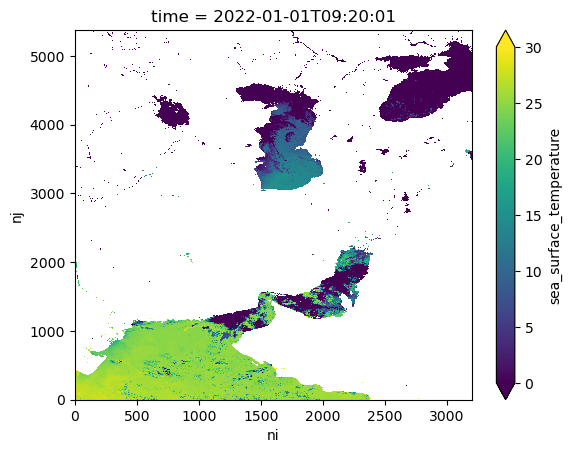
    sea_surface_temperature  (time, nj, ni) float32 ...
    sses_bias                (time, nj, ni) float32 ...
    sses_standard_deviation  (time, nj, ni) float32 ...
    sea_ice_fraction         (time, nj, ni) float32 ...
    l2p_flags                (time, nj, ni) int16 ...
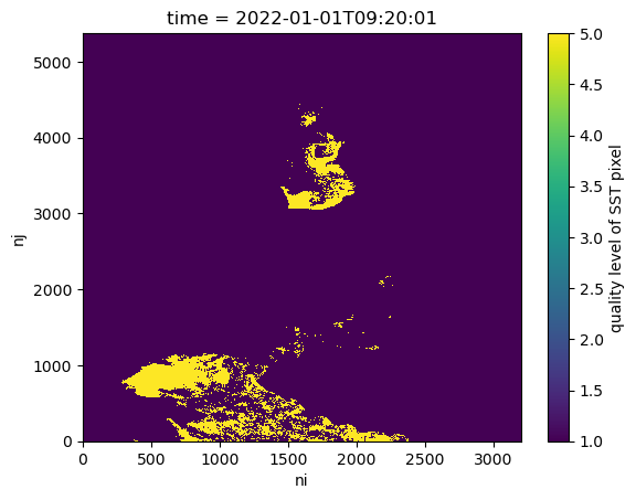
    quality_level            (time, nj, ni) float32 ...
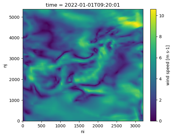
    wind_speed               (time, nj, ni) float32 ...
    sst_gradient_magnitude   (time, nj, ni) float32 ...
    sst_front_position       (time, nj, ni) float32 ...
Attributes: (12/59)
    geospatial_bounds:                        POLYGON((  69.949  53.024,   72...
    geospatial_first_scanline_first_fov_lat:  18.481323
    geospatial_first_scanline_first_fov_lon:  72.716064
    geospatial_first_scanline_last_fov_lat:   14.26062
    geospatial_first_scanline_last_fov_lon:   44.76654
    geospatial_last_scanline_first_fov_lat:   53.02368
    ...                                       ...
    time_coverage_start:                      20220101T092000Z
    title:                                    VIIRS L2P SST
    uuid:                                     fa5182ae-9838-11ec-9306-246e965...
    westernmost_longitude:                    28.064331
    netcdf_version_id:                        4.7.4 of Dec  1 2020 16:57:29 $
    Conventions:                              Conventions = CF-1.7, ACDD-1.3

xarray.Dataset

• Dimensions:
  • time: 1
  • nj: 5376
  • ni: 3200
• Coordinates: (3)
  • time
    (time)
    datetime64[ns]
    2022-01-01T09:20:01

    comment :

    seconds since 1981-01-01 00:00:00

    long_name :

    reference time of sst file

    standard_name :

    time

    axis :

    T

    coverage_content_type :

    coordinate

    array(['2022-01-01T09:20:01.000000000'], dtype='datetime64[ns]')

  • lat
    (nj, ni)
    float32
    ...

    comment :

    Latitude of retrievals

    long_name :

    latitude

    standard_name :

    latitude

    units :

    degrees_north

    valid_max :

    90.0

    valid_min :

    -90.0

    coverage_content_type :

    coordinate

    [17203200 values with dtype=float32]

  • lon
    (nj, ni)
    float32
    ...

    comment :

    Longitude of retrievals

    long_name :

    longitude

    standard_name :

    longitude

    units :

    degrees_east

    valid_max :

    180.0

    valid_min :

    -180.0

    coverage_content_type :

    coordinate

    [17203200 values with dtype=float32]

• Data variables: (12)
  • sst_dtime
    (time, nj, ni)
    timedelta64[ns]
    ...

    comment :

    time plus sst_dtime gives seconds since 1981-01-01 00:00:00 UTC

    long_name :

    time difference from reference time

    valid_max :

    32767

    valid_min :

    -32767

    coverage_content_type :

    referenceInformation

    [17203200 values with dtype=timedelta64[ns]]

  • dt_analysis
    (time, nj, ni)
    float32
    ...

    comment :

    Deviation from reference SST, i.e., dt_analysis = SST - reference SST

    long_name :

    deviation from SST reference

    source :

    CMC0.1deg-CMC-L4-GLOB-v2.0

    units :

    kelvin

    valid_max :

    127

    valid_min :

    -127

    coverage_content_type :

    qualityInformation

    [17203200 values with dtype=float32]

  • satellite_zenith_angle
    (time, nj, ni)
    float32
    ...

    comment :

    satellite zenith angle

    long_name :

    satellite zenith angle

    units :

    degrees

    valid_max :

    32767

    valid_min :

    -32767

    coverage_content_type :

    referenceInformation

    [17203200 values with dtype=float32]

  • sea_surface_temperature
    (time, nj, ni)
    float32
    ...

    comment :

    SST obtained by regression with buoy measurements, sensitive to skin SST. Further information at (Petrenko et al., JGR, 2014; doi:10.1002/2013JD020637)

    long_name :

    sea_surface_subskin_temperature

    source :

    NOAA

    units :

    kelvin

    valid_max :

    32767

    valid_min :

    -200

    standard_name :

    sea_surface_subskin_temperature

    coverage_content_type :

    physicalMeasurement

    [17203200 values with dtype=float32]

  • sses_bias
    (time, nj, ni)
    float32
    ...

    comment :

    Bias is derived against Piecewise Regression SST produced by local regressions with buoys. Subtracting sses_bias from sea_surface_temperature producess more accurate SST at the depth of buoys Further information at (Petrenko et al., JTECH, 2016; doi:10.1175/JTECH-D-15-0166.1)

    long_name :

    SSES bias estimate

    units :

    kelvin

    valid_max :

    127

    valid_min :

    -127

    coverage_content_type :

    qualityInformation

    [17203200 values with dtype=float32]

  • sses_standard_deviation
    (time, nj, ni)
    float32
    ...

    comment :

    Standard deviation of sea_surface_temperature from SST measured by drifting buoys. Further information at (Petrenko et al., JTECH, 2016; doi:10.1175/JTECH-D-15-0166.1)

    long_name :

    SSES standard deviation

    units :

    kelvin

    valid_max :

    127

    valid_min :

    -127

    coverage_content_type :

    qualityInformation

    [17203200 values with dtype=float32]

  • sea_ice_fraction
    (time, nj, ni)
    float32
    ...

    comment :

    Fractional sea ice cover from reference SST

    long_name :

    sea ice fraction

    source :

    CMC0.1deg-CMC-L4-GLOB-v2.0

    standard_name :

    sea_ice_area_fraction

    units :

    1

    valid_max :

    100

    valid_min :

    0

    coverage_content_type :

    auxiliaryInformation

    [17203200 values with dtype=float32]

  • l2p_flags
    (time, nj, ni)
    int16
    ...

    comment :

    L2P common flags in bits 1-6 and data provider flags (from ACSPO mask) in bits 9-16: bit01 (0=IR: 1=microwave); bit02 (0=ocean; 1=land); bit03 (0=no ice; 1=ice); bits04-08 (reserved,set to 0); bit09 (0=radiance valid; 1=invalid); bit10 (0=night; 1=day); bit11 (0=ocean; 1=land); bit12 (0=good quality data; 1=degraded quality data due to "twilight" region); bit13 (0=no glint; 1=glint); bit14 (0=no snow/ice; 1=snow/ice); bits15-16 (00=clear; 01=probably clear; 10=cloudy; 11=clear-sky mask undefined)

    flag_masks :

    [ 1 2 4 256 512 1024 2048 4096 8192 -16384]

    flag_meanings :

    microwave land ice invalid day land twilight glint ice probably_clear_or_cloudy_or_undefined

    long_name :

    L2P flags

    valid_max :

    32767

    valid_min :

    -32768

    coverage_content_type :

    thematicClassification

    [17203200 values with dtype=int16]

  • quality_level
    (time, nj, ni)
    float32
    ...

    comment :

    SST quality levels: 5 corresponds to clear-sky pixels and is recommended for operational applications and validation;

    flag_meanings :

    missing invalid not_used not_used not_used clear

    flag_values :

    [0 1 2 3 4 5]

    long_name :

    quality level of SST pixel

    valid_max :

    5

    valid_min :

    0

    coverage_content_type :

    qualityInformation

    [17203200 values with dtype=float32]

  • wind_speed
    (time, nj, ni)
    float32
    ...

    comment :

    Typically represents surface winds (10 meters above the sea surface)

    height :

    10 m

    long_name :

    wind speed

    standard_name :

    wind_speed

    units :

    m s-1

    valid_max :

    127

    valid_min :

    -127

    source :

    Wind speed from MERRA-2 data

    coverage_content_type :

    auxiliaryInformation

    [17203200 values with dtype=float32]

  • sst_gradient_magnitude
    (time, nj, ni)
    float32
    ...

    valid_min :

    -32767

    valid_max :

    32767

    long_name :

    SST gradient magnitude value

    comment :

    Gradient magnitude calculated from SST field in all grids with valid SST

    units :

    kelvin/km

    coverage_content_type :

    physicalMeasurement

    [17203200 values with dtype=float32]

  • sst_front_position
    (time, nj, ni)
    float32
    ...

    comment :

    Binary indicator of SST front position in the valid SST clear-sky domain: 1 - SST front present, 0 - no front present

    long_name :

    Binary SST front position indicator

    valid_min :

    0

    valid_max :

    1

    coverage_content_type :

    image

    [17203200 values with dtype=float32]

• Indexes: (1)
  • time
    PandasIndex

    PandasIndex(DatetimeIndex(['2022-01-01 09:20:01'], dtype='datetime64[ns]', name='time', freq=None))

• Attributes: (59)

  geospatial_bounds :

  POLYGON(( 69.949 53.024, 72.716 18.481, 44.767 14.261, 28.064 46.733, 69.949 53.024))

  geospatial_first_scanline_first_fov_lat :

  18.481323

  geospatial_first_scanline_first_fov_lon :

  72.716064

  geospatial_first_scanline_last_fov_lat :

  14.26062

  geospatial_first_scanline_last_fov_lon :

  44.76654

  geospatial_last_scanline_first_fov_lat :

  53.02368

  geospatial_last_scanline_first_fov_lon :

  69.94885

  geospatial_last_scanline_last_fov_lat :

  46.733093

  geospatial_last_scanline_last_fov_lon :

  28.064331

  acknowledgement :

  Please acknowledge the use of these data with the following statement: These data were provided by Group for High Resolution Sea Surface Temperature (GHRSST) and the National Oceanic and Atmospheric Administration (NOAA).

  cdm_data_type :

  swath

  comment :

  none

  creator_email :

  Alex.Ignatov@noaa.gov

  creator_name :

  Alex Ignatov

  creator_url :

  http://www.star.nesdis.noaa.gov

  date_created :

  20220228T015142Z

  destripe :

  yes (M5:1.0:f M7:1.0:f M10:1.0:f M12:1.0:b M13:1.0:b M14:1.0:b M15:1.0:b M16:1.0:b)

  easternmost_longitude :

  72.716064

  file_quality_level :

  3

  gds_version_id :

  02.0

  geospatial_lat_resolution :

  0.0067

  geospatial_lat_units :

  degrees_north

  geospatial_lon_resolution :

  0.0067

  geospatial_lon_units :

  degrees_east

  history :

  Created by Advanced Clear-Sky Processor for Oceans (ACSPO)-VIIRS at NOAA/NESDIS/STAR.

  id :

  VIIRS_N20-STAR-L2P-v2.8

  institution :

  NOAA/NESDIS/STAR

  keywords :

  Oceans > Ocean Temperature > Sea Surface Temperature

  keywords_vocabulary :

  NASA Global Change Master Directory (GCMD) Science Keywords

  license :

  GHRSST protocol describes data use as free and open

  metadata_link :

  http://podaac.jpl.nasa.gov/ws/metadata/dataset/?format=iso&shortName=VIIRS_N20-STAR-L2P-v2.8

  naming_authority :

  org.ghrsst

  northernmost_latitude :

  53.11676

  platform :

  N20

  processing_level :

  L2P

  product_version :

  2.80

  project :

  Group for High Resolution Sea Surface Temperature

  publisher_email :

  ghrsst-po@nceo.ac.uk

  publisher_name :

  The GHRSST Project Office

  publisher_url :

  http://www.ghrsst.org

  references :

  Data convention: GHRSST Data Specification (GDS) v2.0. Algorithms: ACSPO-VIIRS ATBD (NOAA/NESDIS/STAR)

  sensor :

  VIIRS

  aggregator_version :

  V1.00

  preprocessor_version :

  1.15.0

  sst_luts :

  LUT_VIIRS_N20_L2P_DEPTH_DAY_V01.05_20201216.txt,

  source :

  VIIRS-MOD-GEO-TC,VIIRS-M5-SDR,VIIRS-M7-SDR,VIIRS-M10-SDR,VIIRS-M12-SDR,VIIRS-M15-SDR,VIIRS-M16-SDR,CMC0.1deg-CMC-L4-GLOB-v2.0,NOAA-NCEP-GFS

  southernmost_latitude :

  14.26062

  spatial_resolution :

  742 m at nadir

  standard_name_vocabulary :

  CF Standard Name Table (v26, 08 November 2013)

  start_time :

  20220101T092000Z

  stop_time :

  20220101T092959Z

  summary :

  Sea surface temperature retrievals produced by NOAA/NESDIS/STAR office from VIIRS sensor

  time_coverage_end :

  20220101T092959Z

  time_coverage_start :

  20220101T092000Z

  title :

  VIIRS L2P SST

  uuid :

  fa5182ae-9838-11ec-9306-246e965ff2b0

  westernmost_longitude :

  28.064331

  netcdf_version_id :

  4.7.4 of Dec 1 2020 16:57:29 $

  Conventions :

  Conventions = CF-1.7, ACDD-1.3

(ds2.sea_surface_temperature-273.15).plot(vmin=0, vmax=30)
plt.show()

ds2.wind_speed.plot()
plt.show()

ds2.quality_level.plot()
plt.show()

base_dir = "../../../data/modis2019/jul21/sst/"
f = os.listdir(base_dir)
print('There are ' + str(len(f)) + ' data files')
for fnm in f[3:7]:
    print(fnm)
    ds_gd=xr.open_dataset(base_dir + fnm, group='geophysical_data')
    ds_gd.sst.plot(vmin=4, vmax=22)
    plt.show()

---------------------------------------------------------------------------
FileNotFoundError                         Traceback (most recent call last)
Cell In[11], line 2
      1 base_dir = "../../../data/modis2019/jul21/sst/"
----> 2 f = os.listdir(base_dir)
      3 print('There are ' + str(len(f)) + ' data files')
      4 for fnm in f[3:7]:

FileNotFoundError: [Errno 2] No such file or directory: '../../../data/modis2019/jul21/sst/'

base_dir = "../../../data/ocean/modis/jul21/sst/"
fnm = 'SNPP_VIIRS.20210722T212401.L2.SST.x.nc'

ds_gd=xr.open_dataset(base_dir + fnm, group='geophysical_data')
ds_nd=xr.open_dataset(base_dir + fnm, group='navigation_data')
ds_nd, ds_gd

---------------------------------------------------------------------------
NameError                                 Traceback (most recent call last)
Cell In[1], line 4
      1 base_dir = "../../../data/ocean/modis/jul21/sst/"
      2 fnm = 'SNPP_VIIRS.20210722T212401.L2.SST.x.nc'
----> 4 ds_gd=xr.open_dataset(base_dir + fnm, group='geophysical_data')
      5 ds_nd=xr.open_dataset(base_dir + fnm, group='navigation_data')
      6 ds_nd, ds_gd

NameError: name 'xr' is not defined

ds_gd.sst.plot(vmin=4.,vmax=22.,xincrease=False)

<matplotlib.collections.QuadMesh at 0x7f78e8cd1950>

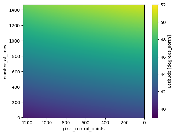
ds_nd.latitude.plot(vmin=39.,vmax=52,xincrease=False)

<matplotlib.collections.QuadMesh at 0x7f78e8baa050>

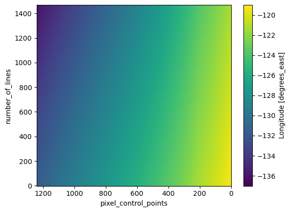
ds_nd.longitude.plot(vmin=-137,vmax=-119,xincrease=False)

<matplotlib.collections.QuadMesh at 0x7f78e8c75310>

ds_sbp = xr.open_dataset(fnm, group='sensor_band_parameters')
ds_sla = xr.open_dataset(fnm, group='scan_line_attributes')
ds_gd = xr.open_dataset(fnm, group='geophysical_data')
ds_nd = xr.open_dataset(fnm, group='navigation_data')

Sort sea surface temperature (SST) datasets by time

• Produces a sorted list of triples: (datetime-string, corresponding datetime64, original filename)

base_dir = "../../../data/ocean/modis/jul21/sst/"
f = os.listdir(base_dir)
sst_files_sorted = []
for fnm in f:
    dtstring = fnm.rstrip('.L2.SST.x.nc')
    if   dtstring[0:12] == 'TERRA_MODIS.': dtstring = dtstring.lstrip('TERRA_MODIS.')
    elif dtstring[0:11] == 'AQUA_MODIS.':  dtstring = dtstring.lstrip('AQUA_MODIS.')
    elif dtstring[0:11] == 'SNPP_VIIRS.':  dtstring = dtstring.lstrip('SNPP_VIIRS.')
    else: 
        print(                              'NON-MATCH filename found ' + fnm)
        break
    expanded_dtstring = dtstring[0:4] + '-' + dtstring[4:6] + '-' + dtstring[6:11] + ':' + dtstring[11:13] + ':' + dtstring[13:15]
    dtvalue = dt64(expanded_dtstring)          # Example: dt64('2017-08-21T07:30:12')
    sst_files_sorted.append((dtstring, dtvalue, fnm))

sst_files_sorted.sort(key=lambda a: a[0])              # Check: print(sst_files_sorted[0], sst_files_sorted[17])

# This cell sets site location lat/lon/depth

eoLat, eoLon, eoDepth     = 44. + 22./60. + 10./3600., -(124. + 57./60. + 15./3600.),  582.
osbLat, osbLon, osbDepth  = 44. + 30./60. + 55./3600., -(125. + 23./60. + 23./3600.), 2906.
axbLat, axbLon, axbDepth  = 45. + 49./60. +  5./3600., -(129. + 45./60. + 13./3600.), 2605.

site_data = {'eo':  { 'name' : 'Endurance Offshore', 'decimal_lat' : eoLat,  'decimal_lon' : eoLon,  'depth' : eoDepth },
             'osb': { 'name' : 'Oregon Slope Base',  'decimal_lat' : osbLat, 'decimal_lon' : osbLon, 'depth' : osbDepth },
             'axb': { 'name' : 'Axial Base',         'decimal_lat' : axbLat, 'decimal_lon' : axbLon, 'depth' : axbDepth }}

print('uh oh... OSB should give 44.52897 -125.38966; check this: ' + str(site_data['osb']['decimal_lat']) + ' ' + str(site_data['osb']['decimal_lon']))

uh oh... OSB should give 44.52897 -125.38966; check this: 44.515277777777776 -125.38972222222223

Southern Hydrate Ridge:      shrLat, shrLon, shrDep       = 44. + 34./60. +  9./3600., -(125  +  8./60. + 53./3600.),  778.
Axial ASHES Vent Field:      ashesLat, ashesLon, ashesDep = 45. + 56./60. +  1./3600., -(130. +  0./60. + 50./3600.), 1543.
Axial Caldera Center:        axcLat, axcLon, axcDep       = 45. + 57./60. + 17./3600., -(130. +  0./60. + 32./3600.), 1528.
Axial Caldera East:          axeLat, axeLon, axeDep       = 45. + 56./60. + 23./3600., -(129. + 58./60. + 27./3600.), 1516.
Axial Caldera International: axiLat, axiLon, axiDep       = 45. + 53./60. + 35./3600., -(129. + 58./60. + 44./3600.), 1520.

# for i in ca: print(i[0], i[1], i[2])
# for i in range(3): for j in range(3): print(m.MODISA_L3m_SST_2014_sst[0][i][j].values)
# 
# testLat = ca[1][1]       #   44.51528
# testLon = ca[1][2]       # -125.38972
# print(testLat, testLon)

sst = []
for i in range(len(ca)):
    # print(m.MODISA_L3m_SST_2014_sst.sel(lat=ca[i][1], lon=ca[i][2], method = 'nearest'))
    temp = modis.MODISA_L3m_SST_2014_sst.sel(lat=ca[i][1], lon=ca[i][2], method = 'nearest').values
    sst.append(round(float(temp[0]), 2))

# Here are MODIS-derived day-time sea surface temperatures at the cabled array locations on 2016-01-01T00:15:10 
print(sst)

Convert line/sample to lat/lon

On this GSFC ocean color page we have details on data groups and format. Quoting:

The data objects in the group geophysical_data are derived from the sensor science data. This group also includes the data quality flags. All of the data objects have dimensions number_of_lines x pixels_per_line. Most parameters are stored as integers, which are scaled according to the attributes scale_factor and add_offset attached to the data object.

Parameters that are wavelength-specific (e.g., Rrs) have separate data objects for each band used to derive the parameter; a list of wavelengths for each sensor provided in the Mission and Sensors entry. The SST and SST4 are stored in separate archive products with their respective quality fields. The specific fields are listed in the Level-2 File Format for each sensor. A complete list of parameters that can be output by the software is given in the L2gen User Guide.

The Level-2 data flags and quality fields are stored in the l2_flags data object in each Level-2 file. This object has attributes flag_masks and flag_meanings that provide the names of the algorithms used in determining the setting of the corresponding bits in l2_flags (the least significant bit being the first bit). The algorithms associated with these names, and the use of the corresponding bits as masks or as flags, are described in volumes of the SeaWiFS TM Series. Note that for SST, only the LAND, SSTWARN and SSTFAIL flags are meaningful, as the quality indicators are stored in sst_qual and sst4_qual, respectively.

Navigation:

The data objects in the group navigation_data contain the geolocation information for the data product. This includes the latitudes and longitudes of the observed locations, the control point indices (needed if the latitudes and longitudes are subsampled and not full-resolution), and the G-ring coordinates for the swath.

nc

ds_gd.sst.plot()

ds.chlor_a.plot()

# bounding box latitude 43 - 47, longitude -123 - -131

datadir = os.getenv("HOME") + "/modis2019/"
datafile = datadir + "A2019283.L3b_DAY_CHL.x.nc"
ds = xr.open_dataset(datafile)
ds
# ds.MODISA_L3b_DAY_CHL.plot(figsize=(12,12))

ds_modis = xr.open_mfdataset()
ds_modis_0 = ds_modis[0]

print(ds_modis_0.MODISA_L3m_SST_2014_sst)
print(ds_modis_0.lat.values[0], modis.lon.values[0], modis.lat.values[-1], modis.lon.values[-1])
modisplot = ds_modis_0.MODISA_L3m_SST_2014_sst.plot(figsize=(12,12))

# bug: This does not work properly yet

# plt.savefig(data + '/images/modis_SST.png')
import matplotlib
img=matplotlib.image.imread(image_d + 'modis_sst.png')
imgplot = plt.imshow(img)
# plt.show()

# The goal is to overlay an image (created earlier; .png file) with a controllable opacity
# 
# How I got to opacity control through a sequence of print statements: 
#   print(thisMap)
#   print(thisMap.layers)
#   print(thisMap.layers[1])                    which is cheating by hardcoding the layer index as 1
#   print(thisMap.layers[1].opacity)
#   therefore setting thisMap.layers[1].opacity = 0.2 works just fine

def ChangeMapOpacity(opacity):thisMap.layers[1].opacity = opacity

from ipyleaflet import Map, ImageOverlay, WMSLayer
opacity = 0.7
thisMap = Map(center=(47, -129), zoom=5, layout=Layout(width='100%', height='600px'))
# The path to the image for overlay is relative; I could not get an absolute path to work...
sourceImage =  '../data/images/modis_sst.png'
image_layer = ImageOverlay(url=sourceImage, bounds=((40.2, -138.58), (53.8, -122.45)), opacity=opacity)
thisMap.add_layer(image_layer)


interact(ChangeMapOpacity, opacity = widgets.FloatSlider(min=0., max=1., step=0.025, value=opacity, 
      continuous_update=False, display='Opacity'))

# It seems that 'thisMap' must be the last line of code in the cell, hence placing interact() above
thisMap

# The following works but does not track zoom with new higher resolution tiles
# wms = WMSLayer(url="https://demo.boundlessgeo.com/geoserver/ows?",layers="nasa:bluemarble")
# thisMap.add_layer(wms)
    



# And this works properly albeit with limited tiling resolution
from ipyleaflet import Map, WMSLayer
wms = WMSLayer(
url="https://demo.boundlessgeo.com/geoserver/ows?",
layers="nasa:bluemarble"
)
m = Map(layers=(wms, ), center=(42.5531, -48.6914), zoom=3)
m

def pp(ds):
    ds['time'] = xr.Variable('time', [pd.Timestamp(ds.attrs['time_coverage_start']) + pd.Timedelta(15, unit='d')])
    return ds

cb=xr.open_mfdataset('modis_chlora_2017_*.nc', preprocess = pp, concat_dim='time').chlor_a.to_dataset()
# cb.chlor_a shows units as mg / cubic meter, numerically equivalent to ug / liter

p,a=plt.subplots(figsize=(13,9))

for x in np.arange(-125.38966-0.1, -125.38966+0.1, 0.1):
    for y in np.arange(44.52897-0.1, 44.52897+0.1, 0.1):
        a.plot(cb.time.values, cb.chlor_a.sel(lon=x, lat=y, method='nearest').values, 'o-')

# cb.to_netcdf('modis_chlora_5_month_timeseries.nc')

cb

latselect = np.arange(44.52897-1., 44.52897+1.00001, 0.10)
lonselect = np.arange(-125.38966-1., -125.38966+1.00001, 0.10)
local = cb.sel(lat = latselect, lon = lonselect, method = 'nearest')
local

%%time
p,a=plt.subplots(figsize=(13,9))
for i in range(9,12):
    for j in range(9,12):
        a.plot(local.time.values, local.chlor_a.isel(lat=i,lon=j).values, 'o-')

a.plot(local.time.values, local.chlor_a.isel(lat=10,lon=10).values, 'o-', linewidth=6)

local.to_netcdf('local.nc')

local=xr.open_dataset('local.nc')
local

l1

# p,a=plt.subplots(figsize=(13,9))
# for t in l1.chlor_a: print(t)  
# a.plot(local.time.values, t.values, 'o-')

for i in range(21): 
    for j in range(21): 
        print(l1.chlor_a[0:5, i, j].values)

local = cb.reindex_like()

local.chlor_a[0].plot(figsize=(14,9),cmap=plt.cm.rainbow,vmin=0.00, vmax=4.0)
plt.xlim(-128,-124); plt.ylim(43.5,45.5); plt.plot(-125.38966, 44.52897, '^')

local.chlor_a[1].plot(figsize=(14,9),cmap=plt.cm.rainbow,vmin=0.00, vmax=4.0)
plt.xlim(-128,-124); plt.ylim(43.5,45.5); plt.plot(-125.38966, 44.52897, '^')

local.chlor_a[2].plot(figsize=(14,9),cmap=plt.cm.rainbow,vmin=0.00, vmax=4.0)
plt.xlim(-128,-124); plt.ylim(43.5,45.5); plt.plot(-125.38966, 44.52897, '^')

local.chlor_a[3].plot(figsize=(14,9),cmap=plt.cm.rainbow,vmin=0.00, vmax=4.0)
plt.xlim(-128,-124); plt.ylim(43.5,45.5); plt.plot(-125.38966, 44.52897, '^')

local.chlor_a[4].plot(figsize=(14,9),cmap=plt.cm.rainbow,vmin=0.00, vmax=4.0)
plt.xlim(-128,-124); plt.ylim(43.5,45.5); plt.plot(-125.38966, 44.52897, '^')

ca=xr.open_rasterio('./chlora.tif').to_dataset(name='chlora')
ca



ca.chlora

cad=ca.where(ca.chlora<1.4)
cad.chlora.plot(figsize=(14,9),cmap=plt.cm.rainbow,vmin=0.00, vmax=1.0)
plt.xlim(-128,-124)
plt.ylim(43.5,45.5)
plt.plot(-125.38966, 44.52897, '^')
# a=p.axes()
# a.set(xlim=(-155,-135))

float(ca.sel(band=0,y=44.52897,x=-125.38966, method='nearest').values)

for x in np.arange(-125.5, -125.0, 0.1):
    for y in np.arange(44.3, 44.8, 0.1):
        print(float(ca.sel(band=0,y=y,x=x, method='nearest').values))