Jupyter Book and GitHub repo.
Data Loader#
The data referenced in this Jupyter Book exceed recommended GitHub repository capacity. As a result this notebook loads data from the cloud as needed to a directory (folder) external to the repository. This directory appears to be part of the repository by means of a symbolic link.
The data source is the interactive oceans zarr-format collections found via the Python s3fs library
under the name ooi-data.
Consequently the data load process can be summarized as ‘I created a data folder with a couple Gigabytes
of available capacity, I set up a symbolic link from within the Jupyter Book oceanography repository
(which I created using git clone); and then I connected to the cloud using the Python s3fs library
to access data of interest.’
The two important preliminary steps (after cloning this repository) are creating that landing space for the data and enabling ingest processing in this notebook/chapter. These steps take about five minutes.
Setting up a landing site for data The repo data folder resides in the
chaptersfolder with a path likedata/rca/sensors/osb. The necessary data volume is about 1GB. Supposer your home directory is/home/roger. The the full path to this folder, assuming you have theoceanographyrepo installed in your home folder, would be/home/roger/oceanography/books/chapters/data/rca/sensors/osb. Notice that this is inside your repository directory. This will work fine as long as you do not have plans to push the repo back to GitHub. Why? Because loading in 1GB of data is considered impolite. To this end you can instead create anosbfolder that is external to the repository and then make a symbolic link to that external folder. An example command sequence:
cd ~
mkdir osb
cd oceanography/book/chapters/data/rca/sensors
rmdir osb
ln -s /home/roger/osb ./osb
This creates a link in your
sensorsfolder that points to the externalosbfolder.
Enable the ingest process: Set
doIngest = Truein the code cell below.
With these two steps done (and presuming you have s3fs installed in your environment)
you are ready to run the cells in this notebook that connect to the sensor stream
datasets. At the moment there are 15 sensors of interest with more pending. One
instrument, the 83-channel spectrophotometer, is treated separately.
Pro tips:
Possible issue if running an ingest cell a second time: The code may try and fail to clobber an existing data file
charting is done from locally saved data, not from cloud data
improvement: charting code ought to check for the local file existence first
improvement: the code should be consolidated as monolithic
For more on Zarr store use see Joe Duprey’s gist on GitHub.
Shallow Profiler Oregon Slope Base January 2022#
import netCDF4
import xarray as xr
import s3fs
from   shallowprofiler  import *
from   charts           import *
from   sys              import exit
from   os               import path
from   time             import time

tic = time()

############################
#####
##### doIngest is a bool code activator: Interact with the zarr data store
#####
############################

doIngest = True

fs = s3fs.S3FileSystem(anon=True)

streamlist = fs.listdir('ooi-data', detail = False)

profiles = ReadProfileMetadata()

# 'streamlist' as the last line of the cell will list out the streams; organized by site and instrument
# For more details on the nomenclature run the following cell.

def InstrumentBreakout(s):
    print('Field breakout:', s[9:11], s[11:13], s[13:15], s[15:17], s[18:20], s[20:22], s[22:23], s[24:26], \
          s[27:32], s[32:33], s[33:36], s[46:])

print('List Oregon Slope Base Profiler streams:\n')
for s in streamlist:
    if 'SF01A' in s: print(s)
print()
print('Translation:')
print('  CTDPF / ctdpf                 CTD')
print('  PHSEN / phsen                 pH')
print('  FLORT / flort                 Fluorometer { FDOM, Chlor-A, Backscatter }')
print('  OPTAA / optaa                 Spectrophotometer')
print('  PARAD / parad                 PAR')
print('  SPKIR / spkir                 Spectral Irradiance')
print('  NUTNR / nutnr_a_dark_sample   Nitrate: Dark sample (explain please)')
print('  NUTNR / nutnr_a_sample        Nitrate: ...')
print('  VELPT / velpt                 Velocity (current) ambiguous: on SCIP or affixed to platform?')
print('  PCO2W / pco2w                 pCO2')
print()

stream_choice = 15       # the 15th element in the file list corresponds to the Shallow Profiler, Oregon Slope Base site

print()
print('Full stream name:', streamlist[stream_choice])
print()
InstrumentBreakout(streamlist[stream_choice])
print()
print('The first field has CE for Coastal Endurance or RS for Regional Cabled Array.')
print('The Oregon Offshore site is a CE site; the other two are RS sites.')
print('Fields 5, 6 and 7 give us shallow profiler site and choice of profiler or platform.')
print()
indenter = 4
print(' '*indenter + 'PC 01 B --> Oregon Offshore 200m Platform')
print(' '*indenter + 'SF 01 B --> Oregon Offshore Profiler')
print(' '*indenter + 'PC 01 A --> Oregon Slope Base 200m Platform')
print(' '*indenter + 'SF 01 A --> Oregon Slope Base Profiler')
print(' '*indenter + 'PC 03 A --> Axial Base 200m Platform')
print(' '*indenter + 'SF 03 A --> Axial Base Profiler')
print()
print('Non-shallow-profiler examples:')
print('  DP O3 A is the Axial Base Deep Profiler')
print('  LJ 01 A is the Oregon Slope Base Seafloor')
print()

def loadData(stream_name):
    fs = s3fs.S3FileSystem(anon=True)
    zarr_store = fs.get_mapper(stream_name)
    ds = xr.open_zarr(zarr_store, consolidated=True)
    return ds

def ShallowProfilerDataReduce(ds, t0, t1, keepers, rename):
    """
    From an XArray Dataset for a shallow profiler instrument stream: Clean up and return a
    subset of the data also in Dataset format.
      - constrain the time range to the interval t0 - t1
      - verify one dimension/coordinate: 'time'
          - others are removed via .drop_dims()
      - from a list of keeper data variables: rename them
      - drop the other data variables
      - drop all the attributes
    """
    if not len(ds.dims) == 1:
        for dim in ds.dims:
            if not dim == 'time':
                ds = ds.drop_dims(dim)
        if not len(ds.dims) == 1: return False, "time dimension only code failed"
    if not list(dict(ds.dims))[0] == 'time':
        return False, "Dataset dim is not 'time' (as assumed)"
    if not len(ds.coords) == 1:
        return False, "Dataset coords count is not 1 (as assumed)"
    if not list(dict(ds.coords))[0] == 'time':
        return False, "Dataset coord is not 'time' (as assumed)"

    ds = ds.sel(time=slice(t0, t1))               # time window

    for s in ds.data_vars:
        if not s in keepers: ds = ds.drop(s)                              # drop extraneous data vars
    for s in ds.data_vars: ds = ds.rename({s:rename[keepers.index(s)]})   # rename the others
    a = [s for s in ds.attrs]
    for p in a: ds.attrs.pop(p)
    return ds, 'looks ok'

osb_profiler_streams = [sname for sname in streamlist if 'SF01A' in sname]

for s in osb_profiler_streams:
    if 'ctdpf' in s: print('CTD:', s)
    if 'velpt' in s: print('Current:', s)

print("There are", len(osb_profiler_streams), "Oregon Slope Base profiler streams")


print(time() - tic, 'seconds\n\n\n')
Jupyter Notebook running Python 3
List Oregon Slope Base Profiler streams:

ooi-data/RS01SBPS-SF01A-2A-CTDPFA102-streamed-ctdpf_sbe43_sample
ooi-data/RS01SBPS-SF01A-2D-PHSENA101-streamed-phsen_data_record
ooi-data/RS01SBPS-SF01A-3A-FLORTD101-streamed-flort_d_data_record
ooi-data/RS01SBPS-SF01A-3B-OPTAAD101-streamed-optaa_sample
ooi-data/RS01SBPS-SF01A-3C-PARADA101-streamed-parad_sa_sample
ooi-data/RS01SBPS-SF01A-3D-SPKIRA101-streamed-spkir_data_record
ooi-data/RS01SBPS-SF01A-4A-NUTNRA101-streamed-nutnr_a_dark_sample
ooi-data/RS01SBPS-SF01A-4A-NUTNRA101-streamed-nutnr_a_sample
ooi-data/RS01SBPS-SF01A-4B-VELPTD102-streamed-velpt_velocity_data
ooi-data/RS01SBPS-SF01A-4F-PCO2WA101-streamed-pco2w_a_sami_data_record

Translation:
  CTDPF / ctdpf                 CTD
  PHSEN / phsen                 pH
  FLORT / flort                 Fluorometer { FDOM, Chlor-A, Backscatter }
  OPTAA / optaa                 Spectrophotometer
  PARAD / parad                 PAR
  SPKIR / spkir                 Spectral Irradiance
  NUTNR / nutnr_a_dark_sample   Nitrate: Dark sample (explain please)
  NUTNR / nutnr_a_sample        Nitrate: ...
  VELPT / velpt                 Velocity (current) ambiguous: on SCIP or affixed to platform?
  PCO2W / pco2w                 pCO2


Full stream name: ooi-data/CE04OSPD-DP01B-04-FLNTUA103-recovered_inst-dpc_flnturtd_instrument_recovered

Field breakout: CE 04 OS PD DP 01 B 04 FLNTU A 103 _inst-dpc_flnturtd_instrument_recovered

The first field has CE for Coastal Endurance or RS for Regional Cabled Array.
The Oregon Offshore site is a CE site; the other two are RS sites.
Fields 5, 6 and 7 give us shallow profiler site and choice of profiler or platform.

    PC 01 B --> Oregon Offshore 200m Platform
    SF 01 B --> Oregon Offshore Profiler
    PC 01 A --> Oregon Slope Base 200m Platform
    SF 01 A --> Oregon Slope Base Profiler
    PC 03 A --> Axial Base 200m Platform
    SF 03 A --> Axial Base Profiler

Non-shallow-profiler examples:
  DP O3 A is the Axial Base Deep Profiler
  LJ 01 A is the Oregon Slope Base Seafloor

CTD: ooi-data/RS01SBPS-SF01A-2A-CTDPFA102-streamed-ctdpf_sbe43_sample
Current: ooi-data/RS01SBPS-SF01A-4B-VELPTD102-streamed-velpt_velocity_data
There are 10 Oregon Slope Base profiler streams
0.5088984966278076 seconds
Go through all 10 osb profiler streams in sequence#
In this order:
ctdpf
phsen
flort
optaa
parad
spkir
nutnr_a_dark_sample
nutnr_a_sample
velpt
pco2w
XXX This Section In Development XXX#
(This code will do the data load as a cycle through the various instruments.)
Scroll down past this to continue: Sequence of instrument-based data loads.
streamlist_profiler_site_keys = {'osb':'SF01A', 'oof':'SF01B', 'axb':'SF03A'}
streamlist_platform_site_keys = {'osb':'PC01A', 'oof':'PC01B', 'axb':'PC03A'}

site_key = 'osb'

profiler_instrument_streams = [sname for sname in streamlist if streamlist_profiler_site_keys[site_key] in sname]
official_instrument_keys = ['ctdpf', 'phsen', 'flort', 'nutnr_a_dark_sample', 'nutnr_a_sample', 'velpt', 'pco2w']
official_unused_instrument_keys =

doIngest = True
do_ingest = [doIngest]*len(instrument_keys)
sensor_official_names = [['corrected_dissolved_oxygen','sea_water_density','sea_water_electrical_conductivity','sea_water_practical_salinity','sea_water_temperature'], \
                         ['ph_seawater'], \
                         ['fluorometric_cdom','fluorometric_chlorophyll_a','optical_backscatter'], \
                         ['nitrate_concentration'], \
                         ['salinity_corrected_nitrate'], \
                         ['velpt_d_upward_velocity','velpt_d_northward_velocity','velpt_d_eastward_velocity'],
                         ['pco2_seawater']]
sensor_informal_names = [['do','density','conductivity','salinity','temp'], ['ph'], ['fdom','chlora','backscatter'], ['nitrate_dark'], ['nitrate'], ['up','north','east'], ['pco2']]
sensor_official_depth = ['sea_water_pressure','int_ctd_pressure','int_ctd_pressure','int_ctd_pressure','int_ctd_pressure','int_ctd_pressure','int_ctd_pressure']

nSensors      = [len(sensorlist) for sensorlist in sensor_official_names]
nSensorsCheck = [len(sensorlist) for sensorlist in sensor_informal_names]
if not nSensors == nSensorsCheck:
    print("Sensor descriptions official/informal do not align")
    exit()
  Cell In[3], line 2
    official_unused_instrument_keys =
                                      ^
SyntaxError: invalid syntax
for ik in instrument_keys:                               # going in order CTD ... pCO2, ik is a string like 'ctdpf'
    idx = instrument_keys.index(ik)                      # idx is an instrument index
    for s in profiler_instrument_streams:                # profiler_instrument_streams is a list of 10 long stream names
        if ik in s:                                      # match up the one we want
            key = profiler_instrument_streams.index(s)   # key is the index of the stream of interest
            print('Found instrument ' + ik + ': ' + s)
            if doIngest[idx]:
                ds = loadData(
                for sensor in sensor_official_names[idx]:
                    sensor_index = sensor_official_names[idx].index(sensor)

            else:
                print("Skipping ingest on this instrument.")
XXX End of In Development Section XXX#
This is the development code
1 of 10: ctdpf i.e. CTD#
tic = time()

for s in osb_profiler_streams:
    if 'ctdpf' in s:
        print('Found CTD:', s)
        stream_ctd = s
        break

if doIngest:
    ds = loadData(stream_ctd)                             # lazy load
    t0, t1 = '2022-01-01T00', '2022-12-31T23'             # January 2022
    ds = ds.sel(time=slice(t0, t1))                       # Subset the full time range to one month
    print(ds.time[0], '              ', ds.time[-1])      # verify selected one month time range
    ds                                                    # get a 'data variable' list of sensors/metadata for this instrument

print(time() - tic, 'seconds\n\n\n')
We pull five sensor time series datasets from the CTD stream. These are named data variables and
they will be renamed using the table found in the Data chapter. Each sensor dataset also contains
time (as dimension/coordinate) and depth (as a second data variable).
Depth is the sea_water_pressure data variable renamed.
corrected_dissolved_oxygen              do              depth
sea_water_density                       density         depth
sea_water_electrical_conductivity       conductivity    depth
sea_water_practical_salinity            salinity        depth
sea_water_temperature                   temp            depth
tic = time()

if doIngest:
    t0, t1 = '2022-01-01T00', '2022-01-31T23'
    ds_do, reply1           = ShallowProfilerDataReduce(ds, t0, t1, ['corrected_dissolved_oxygen', 'sea_water_pressure'], ['do', 'depth'])
    ds_density, reply2      = ShallowProfilerDataReduce(ds, t0, t1, ['sea_water_density', 'sea_water_pressure'], ['density', 'depth'])
    ds_conductivity, reply3 = ShallowProfilerDataReduce(ds, t0, t1, ['sea_water_electrical_conductivity', 'sea_water_pressure'], ['conductivity', 'depth'])
    ds_salinity, reply4     = ShallowProfilerDataReduce(ds, t0, t1, ['sea_water_practical_salinity', 'sea_water_pressure'], ['salinity', 'depth'])
    ds_temp, reply5         = ShallowProfilerDataReduce(ds, t0, t1, ['sea_water_temperature', 'sea_water_pressure'], ['temp', 'depth'])

    if False:
        print(reply1)
        print(reply2)
        print(reply3)
        print(reply4)
        print(reply5)

    if False:
        print(ds_do)
        print(ds_density)
        print(ds_conductivity)
        print(ds_salinity)
        print(ds_temp)

    ds_do.to_netcdf('./data/rca/sensors/osb/do_jan_2022.nc')
    ds_density.to_netcdf('./data/rca/sensors/osb/density_jan_2022.nc')
    ds_conductivity.to_netcdf('./data/rca/sensors/osb/conductivity_jan_2022.nc')
    ds_salinity.to_netcdf('./data/rca/sensors/osb/salinity_jan_2022.nc')
    ds_temp.to_netcdf('./data/rca/sensors/osb/temp_jan_2022.nc')

print(time() - tic, 'seconds\n\n\n')
ds_temp = xr.open_dataset('./data/rca/sensors/osb/temp_jan_2022.nc')

# temperature: ascent versus descent
fig,axs = ChartTwoSensors(profiles, [ranges['temp'], ranges['temp']], [0],
                          ds_temp.temp, -ds_temp.depth, 'T-Ascent',   colors['temp'],    'ascent',
                          ds_temp.temp, -ds_temp.depth, 'T-Descent',  'green',           'descent', 6, 4)
2 of 10: phsen i.e. pH#
if doIngest:
    instrument_key = 'phsen'
    for s in osb_profiler_streams:
        if instrument_key in s:
            print('Found this instrument stream:', s)
            instrument_stream = s
            break

    ds = loadData(instrument_stream)                      # lazy load
    t0, t1 = '2022-01-01T00', '2022-12-31T23'             # January 2022
    ds = ds.sel(time=slice(t0, t1))                       # Subset the full time range to one month
    print(ds.time[0], '              ', ds.time[-1])      # verify selected one month time range
    ds                                                    # get a 'data variable' list of sensors/metadata for this instrument
We pull one sensor time series dataset from this stream. See the CTD section above
and the Data chapter. The data variable of interest is ph_seawater which will be
renamed ph. Depth will be a rename of the int_ctd_pressure data variable.
This stream has multiple dimensions so there is a preliminary step to isolate
just time, ph_seawater and int_ctd_pressure.
if doIngest:
    t0, t1 = '2022-01-01T00', '2022-01-31T23'
    ds_ph, reply = ShallowProfilerDataReduce(ds, t0, t1, ['ph_seawater', 'int_ctd_pressure'], ['ph', 'depth'])
    print(reply)
    print(ds_ph)

    ds_ph.to_netcdf('./data/rca/sensors/osb/ph_jan_2022.nc')
ds_ph = xr.open_dataset('./data/rca/sensors/osb/ph_jan_2022.nc')

# ph: is measured on descent
fig, axes = ChartSensor(profiles, ranges['ph'], [3, 8, 12, 17], ds_ph.ph, -ds_ph.depth, 'profile pH', 'black', 'descent', 6, 4)
3 of 10: flort i.e. fluorometer: Chlor-A, FDOM, particulate backscatter#
if doIngest:
    instrument_key = 'flort'
    for s in osb_profiler_streams:
        if instrument_key in s:
            print('Found this instrument stream:', s)
            instrument_stream = s
            break

    ds = loadData(instrument_stream)                      # lazy load
    t0, t1 = '2022-01-01T00', '2022-12-31T23'             # January 2022
    ds = ds.sel(time=slice(t0, t1))                       # Subset the full time range to one month
    print(ds.time[0], '              ', ds.time[-1])      # verify selected one month time range
    ds                                                    # get a 'data variable' list of sensors/metadata for this instrument
We pull three sensor time series datasets from this stream. See the CTD section above and the Data chapter. Data variables:
fluorometric_cdom           >      fdom, depth
fluorometric_chlorophyll_a  >      chlora, depth
optical_backscatter         >      backscatter, depth
Depth from int_ctd_pressure.
if doIngest:
    t0, t1 = '2022-01-01T00', '2022-01-31T23'
    ds_fdom, reply        = ShallowProfilerDataReduce(ds, t0, t1, ['fluorometric_cdom', 'int_ctd_pressure'], ['fdom', 'depth'])
    ds_chlora, reply      = ShallowProfilerDataReduce(ds, t0, t1, ['fluorometric_chlorophyll_a', 'int_ctd_pressure'], ['chlora', 'depth'])
    ds_backscatter, reply = ShallowProfilerDataReduce(ds, t0, t1, ['optical_backscatter', 'int_ctd_pressure'], ['backscatter', 'depth'])

    ds_fdom.to_netcdf('./data/rca/sensors/osb/fdom_jan_2022.nc')
    ds_chlora.to_netcdf('./data/rca/sensors/osb/chlora_jan_2022.nc')
    ds_backscatter.to_netcdf('./data/rca/sensors/osb/backscatter_jan_2022.nc')
ds_fdom        = xr.open_dataset('./data/rca/sensors/osb/fdom_jan_2022.nc')
ds_chlora      = xr.open_dataset('./data/rca/sensors/osb/chlora_jan_2022.nc')
ds_backscatter = xr.open_dataset('./data/rca/sensors/osb/backscatter_jan_2022.nc')

fig, axes = ChartSensor(profiles, ranges['fdom'],        [0], ds_fdom.fdom,               -ds_fdom.depth,        'profile FDOM', 'blue', 'ascent', 6, 4)
fig, axes = ChartSensor(profiles, ranges['chlora'],      [0], ds_chlora.chlora,           -ds_chlora.depth,      'profile Chlor-A', 'green', 'ascent', 6, 4)
fig, axes = ChartSensor(profiles, ranges['backscatter'], [0], ds_backscatter.backscatter, -ds_backscatter.depth, 'profile backscatter', 'red', 'ascent', 6, 4)
Interpretation: FDOM appears to be a faint or nonexistant signal. Chlorophyll-A shows a strong signal in the mixed layer and then subsides through a cline. Backscatter shows some structure. As above these are single profile charts. Clearly it will be very interesting to view multiple consecutive profiles.
4 of 10: optaa i.e. spectrophotometer 2 signals x 83 channels#
# Not working yet
if False:
    instrument_key = 'optaa'
    for s in osb_profiler_streams:
        if instrument_key in s:
            print('Found this instrument stream:', s)
            instrument_stream = s
            break

    ds = loadData(instrument_stream)                      # lazy load
    t0, t1 = '2022-01-01T00', '2022-12-31T23'             # January 2022
    ds = ds.sel(time=slice(t0, t1))                       # Subset the full time range to one month
    print(ds.time[0], '              ', ds.time[-1])      # verify selected one month time range
    ds                                                    # get a 'data variable' list of sensors/metadata for this instrument
…paused here: This will require unique code to retain the wavelength dimension…
5 of 10: parad i.e. PAR (photosynthetically available radiation)#
if False:
    instrument_key = 'parad'
    for s in osb_profiler_streams:
        if instrument_key in s:
            print('Found this instrument stream:', s)
            print('Compare:                      ooi-data/RS01SBPS-SF01A-3C-PARADA101-streamed-parad_sa_sample')
            instrument_stream = s
            break
if False:
    ds = loadData(instrument_stream)                      # lazy load
    t0, t1 = '2022-01-01T00', '2022-12-31T23'             # January 2022
    ds = ds.sel(time=slice(t0, t1))                       # Subset the full time range to one month
    print(ds.time[0], '              ', ds.time[-1])      # verify selected one month time range
    ds                                                    # get a 'data variable' list of sensors/metadata for this instrument
seems to fail: kernel restart (timeout?)
Compare: Joe says this stream is ok: RS01SBPS-SF01A-3C-PARADA101-streamed-parad_sa_sample and use a bigger machine.
6 of 10: spkir i.e. spectral irradiance#
if False:
    instrument_key = 'spkir'
    for s in osb_profiler_streams:
        if instrument_key in s:
            print('Found this instrument stream:', s)
            instrument_stream = s
            break

    ds = loadData(instrument_stream)                      # lazy load
    t0, t1 = '2022-01-01T00', '2022-12-31T23'             # January 2022
    ds = ds.sel(time=slice(t0, t1))                       # Subset the full time range to one month
    print(ds.time[0], '              ', ds.time[-1])      # verify selected one month time range
    ds                                                    # get a 'data variable' list of sensors/metadata for this instrument
seems to fail: kernel restart (timeout?)
7 of 10: nutnr_a_dark_sample i.e. nitrate explain dark#
if doIngest:
    instrument_key = 'nutnr_a_dark_sample'
    for s in osb_profiler_streams:
        if instrument_key in s:
            print('Found this instrument stream:', s)
            instrument_stream = s
            break

    ds = loadData(instrument_stream)                      # lazy load
    t0, t1 = '2022-01-01T00', '2022-12-31T23'             # January 2022
    ds = ds.sel(time=slice(t0, t1))                       # Subset the full time range to one month
    print(ds.time[0], '              ', ds.time[-1])      # verify selected one month time range
    ds                                                    # get a 'data variable' list of sensors/metadata for this instrument
The dark sample nitrate is on hold pending an explanation of what is going on.
Presuming it was business as usual, maybe: nutnr_nitrogen_in_nitrate becomes nitrate_dark and int_ctd_pressure becomes depth.
if doIngest:
    t0, t1 = '2022-01-01T00', '2022-01-31T23'
    ds_nitrate_dark, reply    = ShallowProfilerDataReduce(ds, t0, t1, ['nitrate_concentration', 'int_ctd_pressure'], ['nitrate_dark', 'depth'])
    ds_nitrate_dark.to_netcdf('./data/rca/sensors/osb/nitrate_dark_jan_2022.nc')

ds_nitrate_dark    = xr.open_dataset('./data/rca/sensors/osb/nitrate_dark_jan_2022.nc')
fig, axes = ChartSensor(profiles, [0, 1],     [3], ds_nitrate_dark.nitrate_dark, -ds_nitrate_dark.depth, 'nitrate (dark)', 'black', 'ascent', 6, 6)
8 of 10: nutnr_a_sample i.e. nitrate#
ds.nitrate_concentration.plot()
ds_nitrate_dark.nitrate_dark.plot()
if doIngest:
    instrument_key = 'nutnr_a_sample'
    for s in osb_profiler_streams:
        if instrument_key in s:
            print('Found this instrument stream:', s)
            instrument_stream = s
            break

    ds = loadData(instrument_stream)                      # lazy load
    t0, t1 = '2022-01-01T00', '2022-12-31T23'             # January 2022
    ds = ds.sel(time=slice(t0, t1))                       # Subset the full time range to one month
    print(ds.time[0], '              ', ds.time[-1])      # verify selected one month time range
    ds                                                    # get a 'data variable' list of sensors/metadata for this instrument
salinity_corrected_nitrate > nitrate and int_ctd_pressure > depth
if doIngest:
    t0, t1 = '2022-01-01T00', '2022-01-31T23'
    ds_nitrate, reply    = ShallowProfilerDataReduce(ds, t0, t1, ['salinity_corrected_nitrate', 'int_ctd_pressure'], ['nitrate', 'depth'])
    ds_nitrate.to_netcdf('./data/rca/sensors/osb/nitrate_jan_2022.nc')

ds_nitrate = xr.open_dataset('./data/rca/sensors/osb/nitrate_jan_2022.nc')
fig, axes = ChartSensor(profiles, ranges['nitrate'], [3], ds_nitrate.nitrate, -ds_nitrate.depth,    'nitrate ', 'black', 'ascent', 6, 6)
9 of 10: velpt i.e. current velocity#
instrument_key = 'velpt'
for s in osb_profiler_streams:
    if instrument_key in s:
        print('Found this instrument stream:', s)
        instrument_stream = s
        break

ds = loadData(instrument_stream)                      # lazy load
t0, t1 = '2022-01-01T00', '2022-12-31T23'             # January 2022
ds = ds.sel(time=slice(t0, t1))                       # Subset the full time range to one month
print(ds.time[0], '              ', ds.time[-1])      # verify selected one month time range
ds                                                    # get a 'data variable' list of sensors/metadata for this instrument
For the current sensor:
depth: int_ctd_pressure. Velocities: velpt_d_upward_velocity, velpt_d_northward_velocity, velpt_d_eastward_velocity.
Respectively depth, up, north, east
if doIngest:
    t0, t1 = '2022-01-01T00', '2022-01-31T23'
    ds_up, reply    = ShallowProfilerDataReduce(ds, t0, t1, ['velpt_d_upward_velocity',    'int_ctd_pressure'], ['up', 'depth'])
    ds_north, reply = ShallowProfilerDataReduce(ds, t0, t1, ['velpt_d_northward_velocity', 'int_ctd_pressure'], ['north', 'depth'])
    ds_east, reply  = ShallowProfilerDataReduce(ds, t0, t1, ['velpt_d_eastward_velocity',  'int_ctd_pressure'], ['east', 'depth'])

    ds_up.to_netcdf('./data/rca/sensors/osb/up_jan_2022.nc')
    ds_north.to_netcdf('./data/rca/sensors/osb/north_jan_2022.nc')
    ds_east.to_netcdf('./data/rca/sensors/osb/east_jan_2022.nc')


ds_up    = xr.open_dataset('./data/rca/sensors/osb/up_jan_2022.nc')
ds_north = xr.open_dataset('./data/rca/sensors/osb/north_jan_2022.nc')
ds_east  = xr.open_dataset('./data/rca/sensors/osb/east_jan_2022.nc')

fig, axes = ChartSensor(profiles, ranges['up'],     [0], ds_up.up,       -ds_up.depth,    'current up', 'black', 'ascent', 6, 4)
fig, axes = ChartSensor(profiles, ranges['north'],  [0], ds_north.north, -ds_north.depth, 'current north', 'black', 'ascent', 6, 4)
fig, axes = ChartSensor(profiles, ranges['east'],   [0], ds_east.east,   -ds_east.depth,  'current east', 'black', 'ascent', 6, 4)
10 of 10: pco2w i.e. pCO2#
if doIngest:
    instrument_key = 'pco2w'
    for s in osb_profiler_streams:
        if instrument_key in s:
            print('Found this instrument stream:', s)
            instrument_stream = s
            break

    ds = loadData(instrument_stream)                      # lazy load
    t0, t1 = '2022-01-01T00', '2022-12-31T23'             # January 2022
    ds = ds.sel(time=slice(t0, t1))                       # Subset the full time range to one month
    print(ds.time[0], '              ', ds.time[-1])      # verify selected one month time range
    ds                                                    # get a 'data variable' list of sensors/metadata for this instrument
descent, midnight and noon pco2_seawater > pco2 and int_ctd_pressure > depth.
if doIngest:
    t0, t1 = '2022-01-01T00', '2022-01-31T23'
    ds_pco2, reply = ShallowProfilerDataReduce(ds, t0, t1, ['pco2_seawater', 'int_ctd_pressure'], ['pco2', 'depth'])
    ds_pco2.to_netcdf('./data/rca/sensors/osb/pco2_jan_2022.nc')

ds_pco2   = xr.open_dataset('./data/rca/sensors/osb/pco2_jan_2022.nc')
fig, axes = ChartSensor(profiles, ranges['pco2'], [3, 8, 12, 17], ds_pco2.pco2,       -ds_pco2.depth,    'pco2', 'black', 'descent', 6, 4)
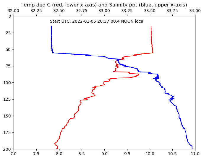
import oceanclient as oc
dfT, dfS = oc.Chart('2022-01-05', 9)
data query result type: <class 'list'> with 8760 elements
prep time 6.17 seconds; data vector length: 4380
dfT, dfS = oc.Chart('2022-01-04', 7)
dfS