Jupyter Book and GitHub repo.
Spectrophotometer#
Introduction#
This notebook concerns the interpretation of data acquired by an ‘AC-S’ spectrophotometer on the Oregon Slope Base shallow profiler. This is a site of the Regional Cabled Array component of the Ocean Observatories Initiative.
The AC-S instrument operates for two intervals each day, each approximately one hour. These are during local midnight and local noon profiler ascents. Two measurements are made across 83 spectral channels: Optical absorption (abbreviated ‘a’) and beam attenuation (denoted ‘c’). The sampling rate is about four samples per second.
To get a sense of the data volume: 7200 seconds per day x 4 samples per second x 2 sample types x 83 channels per sample comes to about 5 million floating point values. In terms of rate of ascent, 3600 seconds corresponds to 180 meters in depth or 5 cm / second.
Ascent = 60 minutes, 180 meters: 300 cm / 60 sec or 5 cm/sec. The vertical bin width used below is 20 cm or 4 sec of data, approximately 16 samples. (Another option: 25 cm or about 20 samples.)
Optical absorbance (\(a\)) is understood to be photon absorption by material in the water column. Beam attenuation (\(c\)) is due to a combination of optical absorption \(a\) and scattering of light \(b\), by seawater and other matter in the water column. \(a \; + \; b \; = \; c\).
For review / revision of this notebook#
Intro corrections + list calculation objectives
\(a\) described as a superposition of multiple signals (Ali)
Short wavelength lamp is low intensity (Ian?): Weak detection; noise; exclude from fit
Mathematics of an exponential fit
Emphasis on DC offsets, indexing wavelenghths vs actual wavelengths, etc
Example: Fitting to wavelength in nm runs aground “1. 1. X”
Review wavelength channels, channel width, overlap
Verify (Chris) wav_a and wav_c correspond to \(a\) and \(c\)
Justify median filter; verify std calculation
Jan thru May 2021 4.2GB
32 Data variables
First redux: 12 days, 2 wavelengths, \(a\) and \(c\)
Second redux: 1 profile March 13 noon local ascent, all channels
Compare Chlor-A from FLORT
Challenge: Eliminate NaN properly
Challenge: Reduce data to depth bins quickly
Still to try: Use the DataFrame method
Document the data size reduction
Extract one representative ascent, all channels, stripped down to A, C for the repo
Attributes are cumbersome
Chart mean for comparison?
Exponential decay fit verify
Truncate both ends?
Comparisons
CDOM proxy to compare to FLORT CDOM (Ali)
ChlorA including 3-point estimate (Chris)
Quenching error tied to PAR
What else?
Part 0. Imports, utilities#
This notebook uses SpectrophotometerModule.py
as well as profiler metadata.
# Set up this notebook to use code from an accompanying Python module file
from SpectrophotometerModule import *
print('\nJupyter Notebook running Python {}'.format(sys.version_info[0]))
---------------------------------------------------------------------------
NameError                                 Traceback (most recent call last)
Cell In[1], line 3
      1 # Set up this notebook to use code from an accompanying Python module file
      2 from SpectrophotometerModule import *
----> 3 print('\nJupyter Notebook running Python {}'.format(sys.version_info[0]))

NameError: name 'sys' is not defined
Part 1. Consolidating source data + load/check#
# For prep see SpectrophotometerModule.py section "Create subset file 1"
s = xr.open_dataset('../RepositoryData/rca/optaa/2021-MAR-13_thru_16_chs_28_and_56.nc')
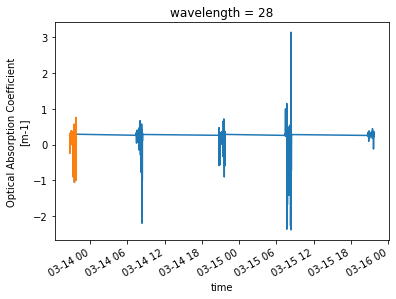
s.oa.sel(wavelength=28).plot()
s.oa.sel(wavelength=28).isel(time=range(14000)).plot()
[<matplotlib.lines.Line2D at 0x7f6768292e50>]
Interpretation#
Use !ls -al to determine this file is 4.3MB. It consists of two wavelengths (channels 28 and 56) and holds both \(a\) and \(c\) data.
There are five profiles shown above spanning 2+ days; again two profile ascents per day. Times shown are in UTC so the first
profile (orange) occurs at local noon on March 13 2021. The ascent runs from 192 to 15 meters depth over one hour.
As a next step we chart \(a\) and \(c\) with depth.
# In profile 'p': index 8 is the first ascent of 2021 where the spectrophotometer collected data
s = xr.open_dataset('../RepositoryData/rca/optaa/2021-MAR-13_thru_16_chs_28_and_56.nc')
channel = 28
day = dt64_from_doy(2021, 72) # March 13
i = GenerateTimeWindowIndices(p, day, day, noon0, noon1)
t0 = p["ascent_start"][i[0]]
t1 = p["ascent_end"][i[0]]
print(t0)
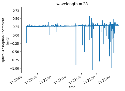
s.sel(wavelength=channel).sel(time=slice(t0, t1)).oa.plot()
2021-03-13 20:42:00
[<matplotlib.lines.Line2D at 0x7f67683e9d60>]
Continuing here with the original program#
Can scroll down to More of the gamma reduction
Part 2. Beam attenuation and optical absorption charts#
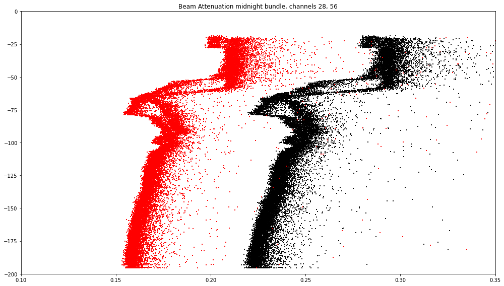
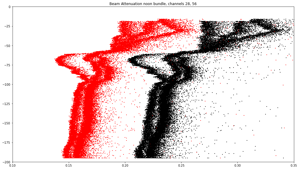
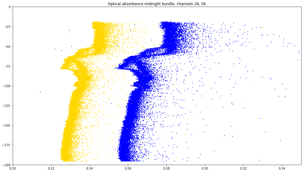
The four charting code blocks below demonstrate overlaying (‘bundle view’) 10 days worth of profiles. These are separated into noon and midnight profiles; and since we have both beam attenuation and optical absorption the total is 2 x 2 = 4 charts.
The work halts here for the moment (with some coding remarks at the bottom) because the data are quite noisy. A single profile takes about 60 minutes; which at 2Hz sampling is 7200 data points. Over ten days this will come to 70k data points per channel. There are about 80 working channels. This sketch is confined to only three of these: 0 (or 1), 40 and 80. So in summary we have four charts with about one million data points and a big gap in the context needed to go further…
pm = GenerateTimeWindowIndices(p, dt64_from_doy(2021, 72), dt64_from_doy(2021, 75), midn0, midn1)
pn = GenerateTimeWindowIndices(p, dt64_from_doy(2021, 72), dt64_from_doy(2021, 75), noon0, noon1)
nm, nn = len(pm), len(pn)

# midnight bundle, beam attenuation
fig, ax = plt.subplots(figsize=(14, 8), tight_layout=True)

for i in range(nm):
    t0, t1 = p["ascent_start"][pm[i]], p["ascent_end"][pm[i]]
    ba =  s.sel(wavelength=28).sel(time=slice(t0,  t1)).ba
    z  = -s.sel(wavelength=28).sel(time=slice(t0, t1)).depth            # z is negated depth to imply below sea surface
    ax.scatter(ba, z, marker=',', s=1., color=colorBA28)               # plot: ax.plot(ba, z, ms = 4., color=colorBA40, mfc=colorBA40)
    ba = s.sel(wavelength=56).sel(time=slice(t0,  t1)).ba
    z  = -s.sel(wavelength=56).sel(time=slice(t0, t1)).depth
    ax.scatter(ba, z, marker=',', s=1., color=colorBA56)

ax.set(title = 'Beam Attenuation midnight bundle, channels 28, 56')
ax.set(xlim = (0.1, 0.35), ylim = (-200, 0.))
plt.show()
# noon bundle, beam attenuation
fig, ax = plt.subplots(figsize=(14, 8), tight_layout=True)

for i in range(nn):
    t0, t1 = p["ascent_start"][pn[i]], p["ascent_end"][pn[i]]
    ba = s.sel(wavelength=28).sel(time=slice(t0,  t1)).ba
    z  = -s.sel(wavelength=28).sel(time=slice(t0, t1)).depth
    ax.scatter(ba, z, marker=',', s=1., color=colorBA28)
    ba = s.sel(wavelength=56).sel(time=slice(t0,  t1)).ba
    z  = -s.sel(wavelength=56).sel(time=slice(t0, t1)).depth
    ax.scatter(ba, z, marker=',', s=1., color=colorBA56)

ax.set(title = 'Beam Attenuation noon bundle, channels 28, 56')
ax.set(xlim = (0.1, 0.35), ylim = (-200, 0.))
plt.show()
# midnight bundle, optical absorbance
fig, ax = plt.subplots(figsize=(14, 8), tight_layout=True)

for i in range(nn):
    t0, t1 = p["ascent_start"][pm[i]], p["ascent_end"][pm[i]]
    oa = s.sel(wavelength=28).sel(time=slice(t0,  t1)).oa
    z  = -s.sel(wavelength=28).sel(time=slice(t0, t1)).depth
    ax.scatter(oa, z, marker=',', s=1., color=colorOA28)
    oa = s.sel(wavelength=56).sel(time=slice(t0,  t1)).oa
    z  = -s.sel(wavelength=56).sel(time=slice(t0, t1)).depth
    ax.scatter(oa, z, marker=',', s=1., color=colorOA56)

ax.set(title = 'Optical absorbance midnight bundle, channels 28, 56')
ax.set(xlim = (0.2, .35), ylim = (-200, 0.))
plt.show()
# noon bundle, optical absorbance
fig, ax = plt.subplots(figsize=(14, 8), tight_layout=True)

for i in range(nn):
    t0, t1 = p["ascent_start"][pn[i]], p["ascent_end"][pn[i]]
    oa = s.sel(wavelength=28).sel(time=slice(t0,  t1)).oa
    z  = -s.sel(wavelength=28).sel(time=slice(t0, t1)).depth
    ax.scatter(oa, z, marker=',', s=1., color=colorOA28)
    oa = s.sel(wavelength=56).sel(time=slice(t0,  t1)).oa
    z  = -s.sel(wavelength=56).sel(time=slice(t0, t1)).depth
    ax.scatter(oa, z, marker=',', s=1., color=colorOA56)

ax.set(title = 'Optical absorbance noon bundle, channels 28, 56')
ax.set(xlim = (0.2, .35), ylim = (-200, 0.))
plt.show()
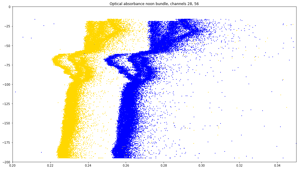
Interpretation#
The noisy nature of the data suggests some filtering. The mixed layer and pycnocline (50 to 75 meter depth) structure suggests building comparison with the March 2021 data found in the BioOptics notebook.
A common data reduction approach is to slice the profile data as depth bins and consider–for each bin–the spectral dimension. Fitting a model of exponential decay will produce a single characteristic paramter \(\large{\gamma}\). These can be stacked with depth.
Begin by fixing depth: We can take the ascent profile and bin the samples to some depth interval. In what follows we us 20 cm intervals, corresponding to about 4 seconds of data acquisition. We expect that wave action would introduce some noise to the signal.
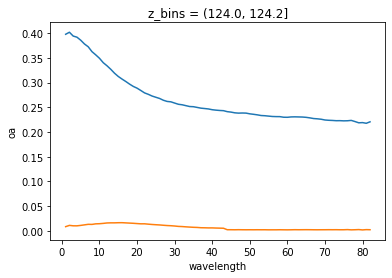
For a given depth bin we can easily calculate four numbers from about 20 samples: \(\normalsize{oa_{mean}, \; oa_{sd}, \; ba_{mean}, \; ba_{sd}}\). All four are charted against wavelength for interest below.
Along the wavelength axis we can fit an exponential curve characterized by a decay constant \(\gamma\).
The decay constant is an indication of particle size distribution. It can be estimated via fit algorithm at each depth bin; and consequently charted against depth.
Gamma reduction#
There are a few items to cover at this point; so this is a temporary section to start some of that.
Further down we have a Mar 13 - Mar 14 time slice giving just one profile ascent
from data file (temporarily) called 04.nc. Time range is 1 hr, 2 min, 42 sec or
3762 seconds. Noon ascent March 13.
2021-03-13T20:42:16.050669056
2021-03-13T21:45:08.062204416
Fit the data to wavelength values
Plot the data with depth axis oriented correctly
Add a box filter version of the signal
Drop Chlorophyll signal onto the same chart using a twin axis
Same: Backscatter
acs=xr.open_dataset("../../data/rca/optaa/20210313.nc")
print(acs.wavelength_a)
wav_a = acs.wavelength_a.copy()
print(wav_a)

# Row 619 of the p[][] DataFrame is the ascent on noon March 13 2021
t0 = p['ascent_start'][619]
t1 = p['ascent_end'][619]

A = xr.open_dataset('../RepositoryData/rca/fluor/osb_chlora_march2021_1min.nc')
B = xr.open_dataset('../RepositoryData/rca/fluor/osb_backscatter_march2021_1min.nc')
C = xr.open_dataset('../RepositoryData/rca/fluor/osb_cdom_march2021_1min.nc')
P = xr.open_dataset('../RepositoryData/rca/par/osb_par_march2021_1min.nc')

A = A.dropna('time')
B = B.dropna('time')
C = C.dropna('time')
P = P.dropna('time')

A=A.sel(time=slice(t0, t1))
B=B.sel(time=slice(t0, t1))
C=C.sel(time=slice(t0, t1))
P=P.sel(time=slice(t0, t1))
<xarray.DataArray 'wavelength_a' (wavelength: 83)>
array([399.6, 403.2, 406.2, 409.3, 413. , 416.6, 420.1, 424.2, 428.6, 432.5,
       436.1, 440. , 444.2, 449. , 453.2, 457.8, 462. , 466.2, 471. , 475.7,
       480.8, 485.3, 489.5, 493.4, 498.1, 502.4, 507.4, 511.8, 517. , 521.3,
       526. , 530.3, 534.7, 538.5, 543.3, 547.5, 552.1, 556. , 560.8, 565.2,
       569.1, 573. , 577.1, 581.2, 583.6, 587.4, 591.8, 596. , 600.6, 605. ,
       609.7, 614.2, 618.4, 623. , 626.7, 631.2, 635. , 639.3, 643.1, 647.4,
       652.4, 656.5, 660.9, 665. , 669.3, 673.6, 677.5, 681.9, 686.1, 689.8,
       693.4, 697.3, 701.2, 704.9, 708.6, 712.3, 716. , 719.5, 723. , 726.8,
       730.7, 734. , 737.8])
Coordinates:
  * wavelength  (wavelength) int32 0 1 2 3 4 5 6 7 8 ... 75 76 77 78 79 80 81 82
Attributes:
    comment:    The wavelength at which optical absorption measurements where...
    precision:  6
    long_name:  Optical Absorption Wavelength
    units:      nm
Plan for what next#
We have t0, t1 defining the time boundaries of the noon ascent on March 13, 2021.
We have datasets A B C P corresponding to Chlor-A, bb700, FDOM, PAR: With NaN removed and focused on this profile. We aim to include Chlor-A on the gamma chart.
Needs attention#
This is the second subset operation: To capture the full spectrum for the full ascent. Needs to go into the Module.
# s = xr.open_dataset("../../data/rca/Spectrophotometer/04.nc")
# s=s.swap_dims({'obs':'time'})
# s.depth.plot()
#
# print('before time select:', s.nbytes)
# s=s.sel(time=slice(t_ascent_0, t_ascent_1))
    # s.time[0] gives 2021-03-13T20:42:16.050669056, s.time[-1] gives 2021-03-13T21:45:08.062204416
    # 14,032 samples in 3772 seconds is 3.72 samples / second x OA / BA x 83 wavelengths
    # s.depth[0], s.depth[-1] gives depth ranging 191.97 to 16.00
# print(' after time select: ', s.nbytes)
# print(s)
#
# s=s.swap_dims({'time':'depth'})
# s=s.sortby('depth')
# s=s.rename({'depth':'z'})
# s

# s=s[['optical_absorption', 'beam_attenuation', 'wavelength_a', 'wavelength_c']]
# s

# s=s.rename({'optical_absorption':'oa','beam_attenuation':'ba'})
# print(s.nbytes)
# s

# s.to_netcdf("../RepositoryData/rca/optaa/march13.nc")
s = xr.open_dataset("../RepositoryData/rca/optaa/2021-MAR-13_noon_full_spectrum.nc")
s
<xarray.Dataset>
Dimensions:       (z: 14032, wavelength: 83)
Coordinates:
    obs           (z) int32 14016 14017 14018 14019 14020 14021 ... 0 5 1 2 3 4
  * wavelength    (wavelength) int32 0 1 2 3 4 5 6 7 ... 75 76 77 78 79 80 81 82
  * z             (z) float64 15.89 15.89 15.89 15.89 ... 192.0 192.0 192.0
Data variables:
    oa            (z, wavelength) float64 ...
    ba            (z, wavelength) float64 ...
    wavelength_a  (wavelength) float64 399.6 403.2 406.2 ... 730.7 734.0 737.8
    wavelength_c  (wavelength) float64 400.1 403.7 406.9 ... 731.5 735.3 738.8
    lat           (z) float64 44.53 44.53 44.53 44.53 ... 44.53 44.53 44.53
    lon           (z) float64 -125.4 -125.4 -125.4 ... -125.4 -125.4 -125.4
    time          (z) datetime64[ns] 2021-03-13T21:45:04.312539648 ... 2021-0...
Attributes: (12/55)
    node:                            SF01A
    comment:
    publisher_email:
    sourceUrl:                       http://oceanobservatories.org/
    collection_method:               streamed
    stream:                          optaa_sample
    ...                              ...
    geospatial_lon_max:              -125.3896636
    geospatial_lon_units:            degrees_east
    geospatial_lon_resolution:       0.1
    geospatial_vertical_units:       meters
    geospatial_vertical_resolution:  0.1
geospatial_vertical_positive: downdz = np.arange(15., 192.2, 0.20) # 886 values, 885 bins: Some will be empty
sm=s.groupby_bins('z', dz).median()
ss=s.groupby_bins('z', dz).std()
sm
<xarray.Dataset>
Dimensions: (z_bins: 885, wavelength: 83)
Coordinates:
* z_bins (z_bins) object (15.0, 15.2] (15.2, 15.4] ... (191.8, 192.0]
* wavelength (wavelength) int32 0 1 2 3 4 5 6 7 ... 75 76 77 78 79 80 81 82
Data variables:
oa (z_bins, wavelength) float64 nan nan nan ... 0.21 0.2142
ba (z_bins, wavelength) float64 nan nan nan ... 0.1167 0.1172
wavelength_a (z_bins, wavelength) float64 nan nan nan ... 730.7 734.0 737.8
wavelength_c (z_bins, wavelength) float64 nan nan nan ... 731.5 735.3 738.8
lat (z_bins) float64 nan nan nan nan ... 44.53 44.53 44.53 44.53
lon (z_bins) float64 nan nan nan nan ... -125.4 -125.4 -125.4def i2z(i): return 15.1 + 0.20*i
def z2i(z): return int((z - 15.0)*5)
sm.oa[z2i(124.0)].plot()
ss.oa[z2i(124.0)].plot()
[<matplotlib.lines.Line2D at 0x7f6765bd5100>]
# from u let's try building sm and ss using the pandas DataFrame method
sm
<xarray.Dataset>
Dimensions: (z_bins: 885, wavelength: 83)
Coordinates:
* z_bins (z_bins) object (15.0, 15.2] (15.2, 15.4] ... (191.8, 192.0]
* wavelength (wavelength) int32 0 1 2 3 4 5 6 7 ... 75 76 77 78 79 80 81 82
Data variables:
oa (z_bins, wavelength) float64 nan nan nan ... 0.21 0.2142
ba (z_bins, wavelength) float64 nan nan nan ... 0.1167 0.1172
wavelength_a (z_bins, wavelength) float64 nan nan nan ... 730.7 734.0 737.8
wavelength_c (z_bins, wavelength) float64 nan nan nan ... 731.5 735.3 738.8
lat (z_bins) float64 nan nan nan nan ... 44.53 44.53 44.53 44.53
lon (z_bins) float64 nan nan nan nan ... -125.4 -125.4 -125.4sm.wavelength_a[19][23]
<xarray.DataArray 'wavelength_a' ()>
array(493.4)
Coordinates:
z_bins object (18.8, 19.0]
wavelength int32 23sm.oa[10]
<xarray.DataArray 'oa' (wavelength: 83)>
array([ nan, 0.41400807, 0.41345352, 0.41002398, 0.406671 ,
0.40507176, 0.39925532, 0.39218378, 0.3868565 , 0.3820011 ,
0.37466399, 0.36786627, 0.36105129, 0.35586958, 0.3491621 ,
0.34402262, 0.33773781, 0.33414286, 0.33054947, 0.32519811,
0.32111595, 0.31683954, 0.31257319, 0.30834062, 0.30455377,
0.30142115, 0.29781416, 0.29421336, 0.29107877, 0.28852163,
0.28639262, 0.28356934, 0.28091301, 0.2791163 , 0.27746933,
0.27588845, 0.27424938, 0.27248608, 0.27099411, 0.26988689,
0.2685633 , 0.26708061, 0.26661129, 0.26600657, 0.26455931,
0.26283272, 0.26149611, 0.26090543, 0.26036225, 0.25905151,
0.2586185 , 0.25709433, 0.25525494, 0.25457033, 0.2538882 ,
0.2528416 , 0.25325943, 0.25227104, 0.25219765, 0.25157741,
0.2519439 , 0.25264334, 0.25390675, 0.25479701, 0.25599931,
0.25541807, 0.25508507, 0.2532454 , 0.25101903, 0.24950096,
0.24682579, 0.24593037, 0.24480865, 0.24337446, 0.24432222,
0.24347339, 0.24421119, 0.2440721 , 0.24195792, 0.24062805,
0.23925863, 0.23743567, 0.23905113])
Coordinates:
z_bins object (17.0, 17.2]
* wavelength (wavelength) int32 0 1 2 3 4 5 6 7 8 ... 75 76 77 78 79 80 81 82n_z_bins = len(sm.z_bins)
n_w_bins = len(sm.wavelength)
sm.wavelength_a[20]
<xarray.DataArray 'wavelength_a' (wavelength: 83)>
array([399.6, 403.2, 406.2, 409.3, 413. , 416.6, 420.1, 424.2, 428.6, 432.5,
       436.1, 440. , 444.2, 449. , 453.2, 457.8, 462. , 466.2, 471. , 475.7,
       480.8, 485.3, 489.5, 493.4, 498.1, 502.4, 507.4, 511.8, 517. , 521.3,
       526. , 530.3, 534.7, 538.5, 543.3, 547.5, 552.1, 556. , 560.8, 565.2,
       569.1, 573. , 577.1, 581.2, 583.6, 587.4, 591.8, 596. , 600.6, 605. ,
       609.7, 614.2, 618.4, 623. , 626.7, 631.2, 635. , 639.3, 643.1, 647.4,
       652.4, 656.5, 660.9, 665. , 669.3, 673.6, 677.5, 681.9, 686.1, 689.8,
       693.4, 697.3, 701.2, 704.9, 708.6, 712.3, 716. , 719.5, 723. , 726.8,
       730.7, 734. , 737.8])
Coordinates:
z_bins object (19.0, 19.2]
* wavelength (wavelength) int32 0 1 2 3 4 5 6 7 8 ... 75 76 77 78 79 80 81 82wav_ref = sm.wavelength_a[0][0:3]
print(wav_ref)
<xarray.DataArray 'wavelength_a' (wavelength: 3)>
array([nan, nan, nan])
Coordinates:
    z_bins      object (15.0, 15.2]
  * wavelength  (wavelength) int32 0 1 2
Put this NaN in the reference and add import curve_fit to the Module#
x = float(nan)
pd.isna(x)
np.isnan(x)
math.isnan(x)
Python: Is not equal to itself: if x != x: will be true if x is NaN
Python: It will not fall within a big range: if float('-inf') < float(num) < float('inf'):
from scipy.optimize import curve_fit
def func(x, a, b, c): return a * np.exp(-b * x) + c


gamma, depth = [], []

for i in range(n_z_bins):

    if not i%20: print(i)

    oa, wav = [], []
    for j in range(n_w_bins):
        if not pd.isna(float(sm.oa[i][j])):
            oa.append(float(sm.oa[i][j]))
            wav.append(float(sm.wavelength_a[i][j])-403.2)

    # print(len(oa), len(wav))
    # print(len(oa), len(wav), oa[20], wav[20])
    # print(type(oa))
    # plt.plot(wav, oa)

    if len(oa) > 3:
        popt, pcov = curve_fit(func, wav, oa)
        # print(len(oa), len(wav), popt)
        gamma.append(popt[1])
        depth.append(-i2z(i))

plt.plot(gamma, depth)
0
20
40
60
80
100
120
140
160
180
200
220
240
260
280
300
320
340
360
380
400
420
440
460
480
500
520
540
560
580
600
620
640
660
680
700
720
740
760
780
800
820
840
860
880
[<matplotlib.lines.Line2D at 0x7f675e8f55b0>]
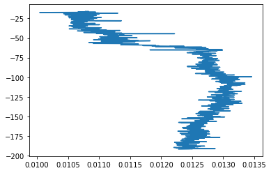
plt.plot(gamma, depth)
[<matplotlib.lines.Line2D at 0x7f675e418370>]
def smooth(y, n):
'''
Boxcar smoothing; it assumes x-spacing even
'''
r, idx = [], []
for i in range(0, len(y)):
ii, jj, s, np = max(i - n, 0), min(i + n, len(y)-1), 0, 0
for k in range(ii, jj + 1):
if y[k] > 0.: s, np = s + y[k], np + 1
if np:
r.append(s/np)
idx.append(i)
return r, idx
g_s, i_s = smooth(gamma, 5)
fig,ax=plt.subplots(figsize=(8,8),tight_layout=True)
atA = ax.twiny()
# atP = ax.twiny()
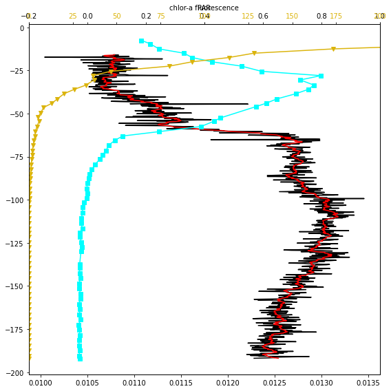
ax.plot(gamma, depth, color='k')
ax.plot(g_s, depth, color='r')
atA.set_xlabel('chlor-a fluorescence', color='k')
atA.plot(A.chlora, A.z, marker='s', markersize = 6., color='cyan', markerfacecolor='cyan')
atA.tick_params(axis='x', labelcolor='k')
atA.set(xlim = (-0.2, 1.0))
if False:
atB = ax.twiny()
atB.set_xlabel('bb700', color='k')
atB.plot(B.backscatter, B.z, marker='s', markersize = 6., color='magenta', markerfacecolor='magenta')
atB.tick_params(axis='x', labelcolor='magenta')
atB.set(xlim = (0., .002))
atP = ax.twiny()
atP.set_xlabel('PAR', color='k')
atP.plot(P.par, P.z, marker='v', markersize = 6., color='xkcd:gold', markerfacecolor='xkcd:gold')
atP.tick_params(axis='x', labelcolor='xkcd:gold')
atP.set(xlim = (0., 200.))
plt.show()
A
<xarray.Dataset>
Dimensions:  (time: 65)
Coordinates:
  * time     (time) datetime64[ns] 2021-03-13T20:42:00 ... 2021-03-13T21:48:00
Data variables:
    chlora   (time) float64 -0.02483 -0.028 -0.02631 ... 0.245 0.2141 0.184
    z        (time) float64 -192.0 -190.5 -187.5 -184.5 ... -12.5 -9.5 -7.5
Attributes: (12/44)
    cdm_altitude_proxy:            z
    cdm_data_type:                 TimeSeriesProfile
    cdm_profile_variables:         time
    cdm_timeseries_variables:      station,longitude,latitude
    contributor_email:             feedback@axiomdatascience.com
    contributor_name:              Axiom Data Science
    ...                            ...
    standard_name_vocabulary:      CF Standard Name Table v72
    station_id:                    104289
    summary:                       Timeseries data from 'Regional Cabled Arra...
    time_coverage_end:             2021-08-02T23:59:00Z
    time_coverage_start:           2014-10-06T14:10:00Z
title: Regional Cabled Array: Oregon Slope Base S...Move this to reference: How to fit to an exponential#
Need to resolve the “fit to x relative to x0” business.
import matplotlib.pyplot as plt

from scipy.optimize import curve_fit

def func(x, a, b, c): return a * np.exp(-b * x) + c

xdata = np.linspace(0, 4, 50)

y = func(xdata, 2.5, 1.3, 0.5)
rng = np.random.default_rng()

# null hypothesis produces gamma = 1.3 as desired
# y_noise = [0.]*len(xdata)
y_noise = 0.2 * rng.normal(size=xdata.size)

ydata = y + y_noise
print(type(ydata))

popt, pcov = curve_fit(func, xdata, ydata)
print(popt[1], type(popt[1]))
Move to ref with the cell above#
fig,ax = plt.subplots(figsize=(6, 4), tight_layout=True)
ax.plot(xdata, func(xdata, *popt), 'r-', label='fit: a=%5.3f, b=%5.3f, c=%5.3f' % tuple(popt))
plt.plot(xdata, ydata, 'b-', label='data')
plt.xlabel('x')
plt.ylabel('y')
plt.legend()
plt.show()
Code fragments#
The following code pertains to multi-plot building, data subsets and interactive views of the data. It should be relocated out of this notebook to the reference material.
# declaring figure and axes
# fig, axs = plt.subplots(fig_n_down, fig_n_across, figsize=(fig_width * fig_n_across, fig_height*fig_n_down), tight_layout=True)

# referencing one of these axes
# axs[day_index][3]

# using index selection
# .isel(wavelength=oa_plot_wavelength)

################################
# interact example
################################

# intro text:
# We have two charts per day (midnight and noon) and two observation types (OA and BA). This is 2 x 2 charts.
#   The display is 2 such blocks, left and right, for 4 x 2 charts. When the checkbox is True we use the passed
#   values for the right chart and the stored values for the left. When the checkbox is False we use the passed
#   values for the left chart and the stored values for the right. In either case the updated states are stored
#   in global state variables. If the day is 0 there is no plot. A four-chart state is { day_ba, day_oa, channel_oa }.

# sliders etc set up:
# interact(spectrophotometer_display, \
#          sel_day_ba=widgets.IntSlider(min=1, max=31, step=1, value=9,  continuous_update=False, description='BAtten'),
#          sel_day_oa=widgets.IntSlider(min=1, max=31, step=1, value=9,  continuous_update=False, description='OAbs'),
#          sel_channel_oa=widgets.IntSlider(min=1, max=82, step=1, value=49,  continuous_update=False, description='OA Chan'),
#          right = widgets.ToggleButton(value=False, description='use right charts', disabled=False,
#              button_style='', tooltip='Description', icon='check')
#     )

# corresponding function:
# def spectrophotometer_display(sel_day_ba, sel_day_oa, sel_channel_oa, right):
Part 3. Residual notes#
AC-S on the Oregon Slope Base shallow profiler: midnight and noon ascents
First is 7:22 Zulu: midnight off the coast of Oregon
RCA shallow profilers execute nine profiles per day from 200m to 5m nominal depths
Ascent duration is an hour
Nitrate measures on descent
The ascent minimum depth is five meters but is typically more, varying with sea conditions
AC-S: optical absorption (OA), beam attenuation (BA)
With time and pressure in dbar; depth in m
Instrument sampling rate is ~3.7 samples per second
Instrument records 86 spectral channels
Light wavelength is ~(400nm + channel number x 4nm)
Channel width is ~20nm so channels overlap
Signals shift with wavelength
Channels 0, 83, 84 and 85 tend to give
nanvalues (not usable) for both OA and BATend to use channels 2 through 82
Both OA and BA data are idiosyncratic
The midnight OA data are quantized in a peculiar manner; see charts below
The noon OA are somewhat quantized but have more reasonable / data-like structure
BA data are not fraught with the OA quantization issue
Both midnight and noon BA data include substantial noise
Variance is also apparent in BA data
This suggests filtering by depth bin and possibly discarding outliers
Un-answered questions
Is this particular time interval simply ‘instrument fail’?
Why are OA data different in midnight versus noon profiles?
Are OA and BA typically combined into a turbidity value?
What wavelength ranges are of particular interest?
How do these signals compare with fluorometers, nitrate, CTD, pH, etcetera?
OOI site has SME remarks circa 2016 (not illuminating)
References from OOI
Paraphrasing the Subject Matter Export evaluation (link above):
Dr. Boss (SME) verified 1.5 months of data (April-May 2015): Processing and plotting data using the raw data and vendor calibration files from the AC-S, salinity and temperature from a collocated CTD data to correct absorption and attenuation median spectra and scattering, and data from a collocated fluorometer to cross-check the chlorophyll and POC results.
Consistency between the sensors suggests that they did not foul during the deployment. Not only did his results show that accurate data was being produced by all the sensors in question, but the AC-S (an extremely sensitive instrument normally deployed for very short periods of time) did not drift noticeably during the deployment period, a notable achievement.
Paraphrased from the sheet on Optical Absorption (OA):
The OPTAA is a WET Labs AC-S spectral absorption and attenuation meter. Total wavelength span is 400–750 nm in approximately 4 nm steps. Individual filter steps (channels) have a full-width half maximum response between about 10 to 18 nm.
35 OPTAA instruments are deployed throughout the initial OOI construction: Pioneer, Endurance, Regional and Global arrays.
Depends on a calibrated instrument as well as water temperature and practical salinity derived from a co-located and synchronized CTD.
While small corrections for salinity are available at visible wavelengths (< 700 nm), temperature and salinity corrections are more significant at infrared wavelengths (> 700 nm) and must be performed on both the absorption and attenuation signals.
The beam attenuation (BA) sheet is similar. Both give a mathematical basis for the data as well as code.