Jupyter Book and GitHub repo.
Anomaly and Coincidence#
This notebook generates anomaly metadata for an OOI RCA shallow profiler, typically scanning a time series lasting one month. This anomaly scan is based on a calculated threshold deviation. As we have multiple sensors types, coincident anomalies are particularly interesting. Here are some initial questions.
What anomaly patterns emerge?
How might anomalies be interpreted in spatial extent terms (as we also have current data at the fixed profiler sites)
Can auxiliary data resources corroborate or expand our view of the ocean behavior?
Tactical approach#
Build a data dictionary d{} from existing shallow profiler data
For each sensor: Average data as a function of depth to create reference profiles
A typical month with 31 days would have 31 x 9 = 279 profiles to average
Profile data are downsampled to one sample per minute, ~3 meter vertical bins
For each sensor create a two dimensional scalar field: An ‘anomaly map’
‘vertical axis’ is depth
‘horizontal axis’ is profile index, i.e. time over the course of the chosen month
scalar value is (data - reference mean) / reference standard deviation
From a visual look at anomaly maps we can evaluate the premise of anomalies and sharp anomalies.
Sensor phases#
The CTD-associated sensors have the highest data density (samples per unit distance in depth per unit time) and are relegated to ‘phase one’of the anomaly calculation process. These include conductivity, density, salinity, temperature, dissolved oxygen concentration, and three types of measurement from the fluorometer triplet: Chlorophyll-A, FDOM and particulate backscatter.
Note: The five CTD values { C, D, S, T, Z } are not entirely independent
The second phase concerns sensors that operate on only the midnight and noon profiles (two of the nine daily profiles): pH, pCO2 and nitrate concentration.
The third phase concerns ambient light measurement: PAR and the seven spectral irradiance bands.
The fourth phase concerns the spectrophotometer: Optical absorbance and beam attenuation across approximately 80 spectral bands.
Phase 1#
from shallowprofiler import ReadProfileMetadata, sensors, ranges, standard_deviations, colors, sensor_names, DataFnm
from charts import ChartTwoSensors
from anomaly import *

# profiles is a pandas DataFrame treated as a global resource
month_choice = 'jan22'
profiles = ReadProfileMetadata('../profiles/osb_profiles_' + month_choice + '.csv')
Jupyter Notebook running Python 3
---------------------------------------------------------------------------
ImportError                               Traceback (most recent call last)
Cell In[1], line 1
----> 1 from shallowprofiler import ReadProfileMetadata, sensors, ranges, standard_deviations, colors, sensor_names, DataFnm
      2 from charts import ChartTwoSensors
      3 from anomaly import *

ImportError: cannot import name 'DataFnm' from 'shallowprofiler' (/home/runner/work/oceanography/oceanography/book/chapters/shallowprofiler.py)
d = {}

for sensor in sensors:
    if not sensor[0] == 'spkir':
        d[sensor[0]] = (xr.open_dataset(DataFnm('osb', sensor[1], month_choice, sensor[0]))[sensor[0]],
                        xr.open_dataset(DataFnm('osb', sensor[1], month_choice, sensor[0]))['z'],
                        ranges[sensor[0]][0], ranges[sensor[0]][1], colors[sensor[0]])
    else:
        waves = ['412nm', '443nm','490nm','510nm','555nm','620nm','683nm']
        for wave in waves:
            d[wave] = (xr.open_dataset(DataFnm('osb', 'spkir', month_choice, 'spkir'))[wave],
                       xr.open_dataset(DataFnm('osb', 'spkir', month_choice, 'spkir'))['z'],
                       ranges['spkir'][0], ranges['spkir'][1], colors['spkir'])
# So now we have d['density'] and so forth: So print the keys of this dictionary
for da in d: print(da)

sensors_phase1 = ['conductivity', 'density', 'salinity', 'temperature', 'do', 'chlora', 'bb', 'fdom']
sensors_phase2 = ['nitrate', 'pco2', 'ph']
sensors_phase3 = ['par', '412nm', '443nm', '490nm', '510nm', '555nm', '620nm', '683nm']
sensors_phase4 = ['oa', 'ba']
# vel is handled independently
conductivity
density
pressure
salinity
temperature
chlora
bb
fdom
412nm
443nm
490nm
510nm
555nm
620nm
683nm
nitrate
pco2
do
par
ph
up
east
north
# a reminder of the 5-tuple dictionary d
print(d['temperature'][0].name)
print(d['temperature'][1].name)
print(d['temperature'][2])
print(d['temperature'][3])
print(d['temperature'][4])

print(type(d['temperature'][1]))
temperature
z
7
14
red
<class 'xarray.core.dataarray.DataArray'>
# Flag: Move these charting functions to charts.py
# flag bug no markers are displayed
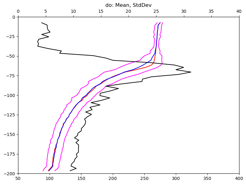
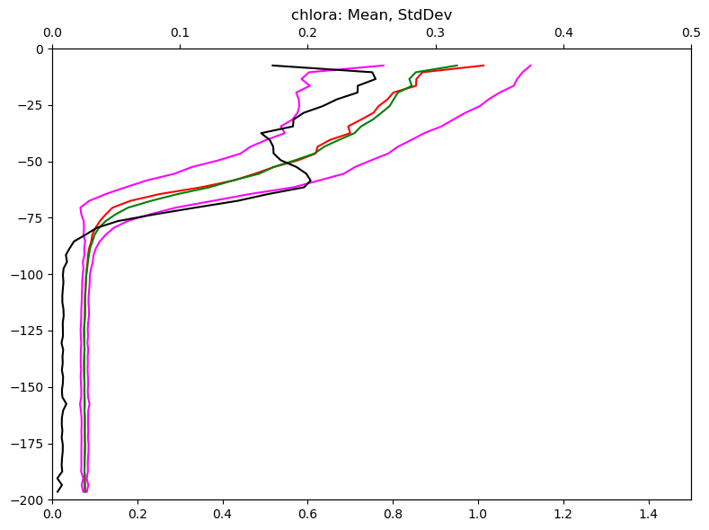
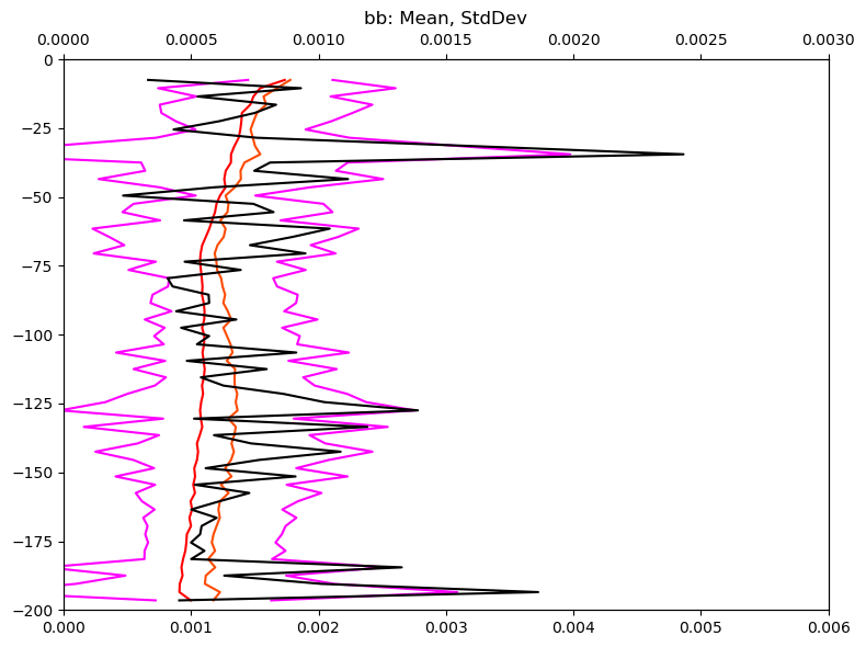
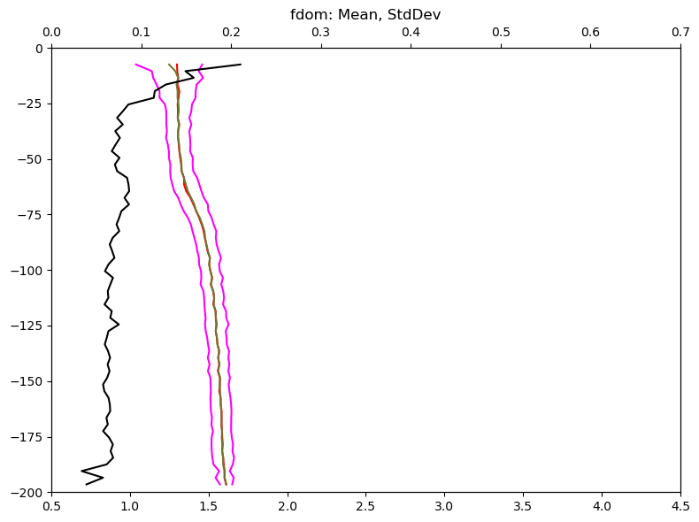
def ChartMeanStdDev(name, ranges, daM, daSD, wid, hgt, colorM, colorSD):
'''Strictly mean and standard deviation'''
fig, ax = plt.subplots(figsize=(wid, hgt), tight_layout=True)
axtwin = ax.twiny()
sdcol = 'magenta'
ax.plot( daM, daM['z'], ms = 4., color=colorM, mfc=colorM)
ax.plot( daM + daSD, daM['z'], ms = 10., color=sdcol, mfc='red')
ax.plot( daM - daSD, daM['z'], ms = 10., color=sdcol, mfc='red')
axtwin.plot(daSD, daSD['z'], ms = 4., color=colorSD, mfc=colorSD)
z0, z1 = -200., 0.
ax.set( xlim = (ranges[0][0], ranges[0][1]), ylim = (z0, z1))
axtwin.set(xlim = (ranges[1][0], ranges[1][1]), ylim = (z0, z1))
ax.set(title=name + ': Mean, StdDev')
return
def ChartMeanStdDevMedian(name, ranges, daM, daSD, daMed, wid, hgt, colorM, colorSD):
'''Mean, standard deviation and also median'''
fig, ax = plt.subplots(figsize=(wid, hgt), tight_layout=True)
axtwin = ax.twiny()
sdcol = 'magenta'
ax.plot( daMed, daMed['z'], ms = 4., color='red', mfc=colorM)
ax.plot( daM, daM['z'], ms = 4., color=colorM, mfc=colorM)
ax.plot( daM + daSD, daM['z'], ms = 10., color=sdcol, mfc='red')
ax.plot( daM - daSD, daM['z'], ms = 10., color=sdcol, mfc='red')
axtwin.plot(daSD, daSD['z'], ms = 4., color=colorSD, mfc=colorSD)
z0, z1 = -200., 0.
ax.set( xlim = (ranges[0][0], ranges[0][1]), ylim = (z0, z1))
axtwin.set(xlim = (ranges[1][0], ranges[1][1]), ylim = (z0, z1))
ax.set(title=name + ': Mean, StdDev')
return
Development code for understanding a sensors profile with depth#
Note the placeholder remark on a low-pass filter.
# Using depth bins ('z') compute means and standard deviations
n_meters = 200
n_meters_per_bin = 2
bin_upper_zs = np.linspace(-n_meters, 0,1 + int(n_meters/n_meters_per_bin))
bin_upper_zs
sensor_name = 'temperature'
dd = d[sensor_name] # tuple (DataArray, DataArray, range0, range1, color
print(dd[0].name)
print(dd[1].name)
print(dd[2])
print(dd[3])
print(dd[4])
ds = xr.merge([dd[0], dd[1]]) # accepts a list of DataArrays
ds = ds.swap_dims({'time':'z'})
ds = ds.drop('time')
dsM = ds.groupby_bins('z', bin_upper_zs).mean()
dsSD = ds.groupby_bins('z', bin_upper_zs).std()
dsC = ds.groupby_bins('z', bin_upper_zs).count()
dsM=dsM.assign_coords(z_bins=np.array([v.mid for v in dsM.z_bins.values])).rename({'z_bins': 'z'})
dsSD=dsSD.assign_coords(z_bins=np.array([v.mid for v in dsSD.z_bins.values])).rename({'z_bins': 'z'})
dsC=dsC.assign_coords(z_bins=np.array([v.mid for v in dsC.z_bins.values])).rename({'z_bins': 'z'})
dsM['z'][0:30]
# flag a low pass filter would go here
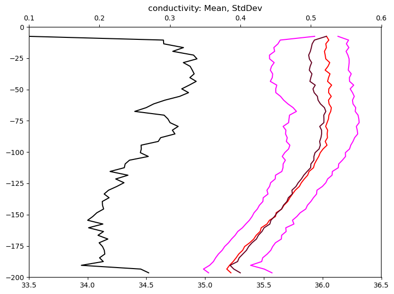
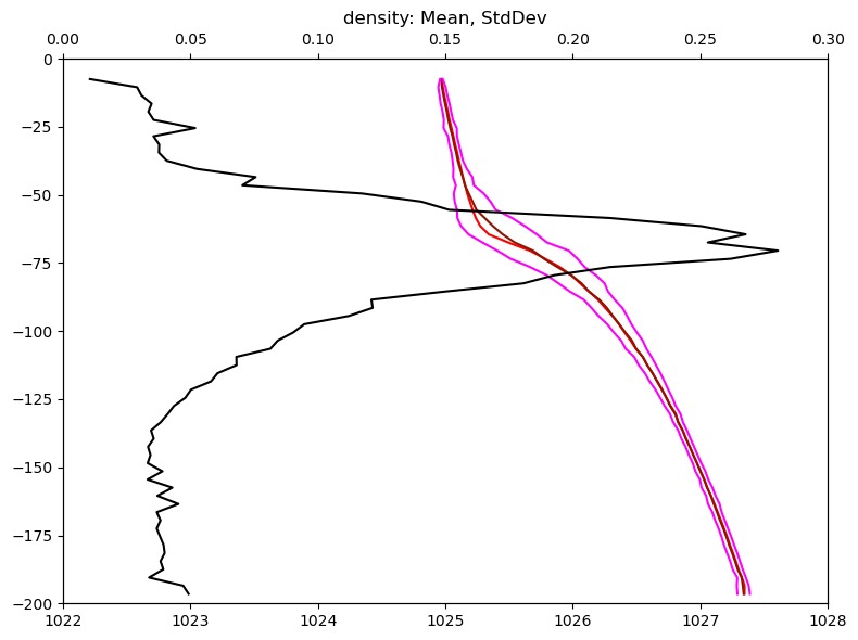
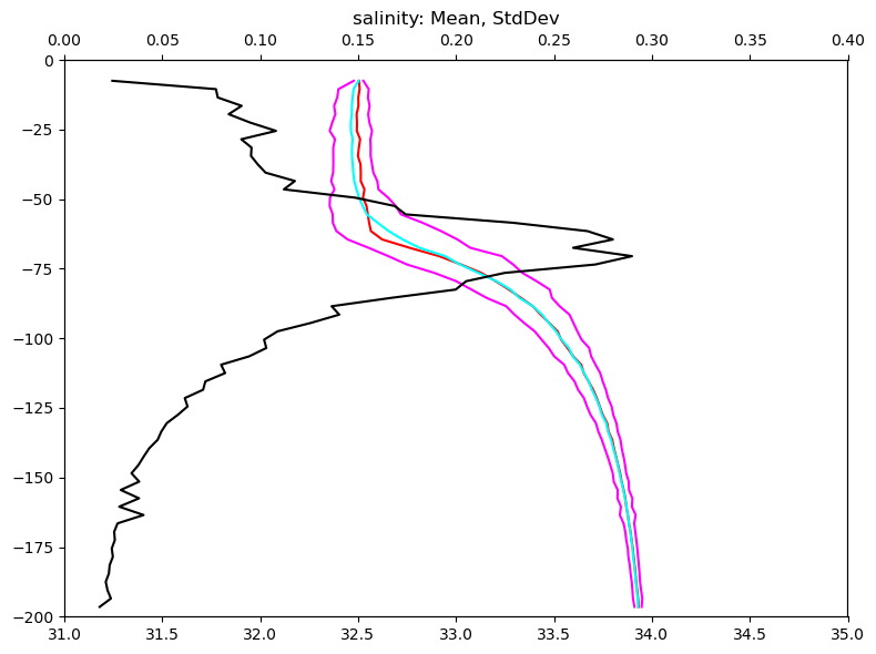
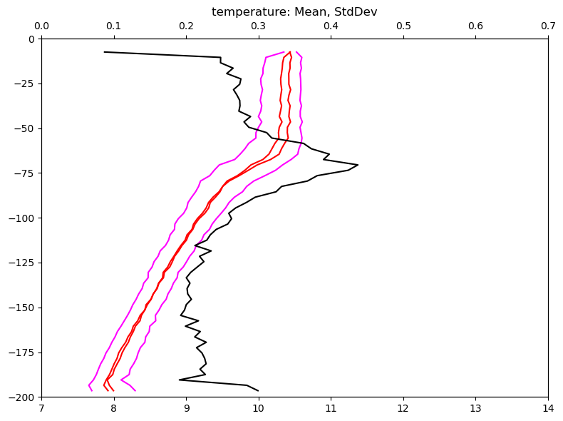
ChartMeanStdDev(sensor_name, [ranges[sensor_name],standard_deviations[sensor_name]], dsM[sensor_name], dsSD['stddev'], 10, 8, dd[4], 'black')
Example of seaborn for relative magnitude charting#
import seaborn as sns

x = np.array([1, 1, 1, 1, 2, 2, 2, 2, 3, 3, 3, 3])
y = np.array([1, 2, 3, 4, 1, 2, 3, 4, 1, 2, 3, 4])
z = np.array([249, 523, 603, 775, 577, 763, 808, 695, 642, 525, 795, 758])
df = pd.DataFrame({'x':x, 'y':y, 'z':z})

sns.relplot(data=df, x='x', y='y', size='z', sizes=(10, 100), hue='z', palette='coolwarm',)
Compile a dictionary of reference profiles (mean, stddev, count)#
# r1 will be the phase-1 *r*eference dictionary
#  tuple of 3 data arrays: mean, stddev, count (all three include depth dimension/coord z)
#  the upper depth is zero
#  the lower depth is <= -200 and is chosen to give an integer bin count

n_zone_meters     = 201
n_meters_per_bin  = 3
bin_upper_zs      = np.linspace(-n_zone_meters + n_meters_per_bin, 0, n_zone_meters//n_meters_per_bin)

r1 = {}                                      # r1 will be a dictionary of triples ( , , )
for sensor_name in sensors_phase1:
    dd     = d[sensor_name]                    # 5-tuple (DataArray, DataArray, range0, range1, color
    ds     = xr.merge([dd[0], dd[1]])
    ds     = ds.swap_dims({'time':'z'})
    ds     = ds.drop('time')
    dsM    = ds.groupby_bins('z', bin_upper_zs).mean()
    dsM    = dsM.assign_coords(z_bins=np.array([v.mid for v in dsM.z_bins.values])).rename({'z_bins': 'z'})
    dsSD   = ds.groupby_bins('z', bin_upper_zs).std()
    dsSD   = dsSD.assign_coords(z_bins=np.array([v.mid for v in dsSD.z_bins.values])).rename({'z_bins': 'z'}).rename({sensor_name: 'stddev'})
    dsC    = ds.groupby_bins('z', bin_upper_zs).count()
    dsC    = dsC.assign_coords(z_bins=np.array([v.mid for v in dsC.z_bins.values])).rename({'z_bins': 'z'}).rename({sensor_name: 'count'})
    dsMed  = ds.groupby_bins('z', bin_upper_zs).median()
    dsMed  = dsMed.assign_coords(z_bins=np.array([v.mid for v in dsMed.z_bins.values])).rename({'z_bins': 'z'}).rename({sensor_name: 'median'})
    r1[sensor_name] = (dsM[sensor_name], dsSD['stddev'], dsC['count'], dsMed['median'])
    ChartMeanStdDevMedian(sensor_name, [ranges[sensor_name], standard_deviations[sensor_name]], dsM[sensor_name], dsSD['stddev'], dsMed['median'], 8, 6, dd[4], 'black')
dd = d['temperature'] # 5-tuple (DataArray, DataArray, range0, range1, color
ds = xr.merge([dd[0], dd[1]]) # note that dd[0] does not include z; so we refer to dd[1]
ds = ds.swap_dims({'time':'z'})
ds = ds.drop('time')
dsMed = ds.groupby_bins('z', bin_upper_zs).median()
dsMed = dsMed.assign_coords(z_bins=np.array([v.mid for v in dsMed.z_bins.values])).rename({'z_bins': 'z'}).rename({'temperature': 'median'})
#### Verify reference generation agrees with a traditional means of calculation
# let's do temperature old school and make sure it looks the same
tt=d['temperature'][0].data
tz=d['temperature'][1].data
# ndarrays: print(type(tt), type(tz)); tt.shape gives (44638,)
tdata = list(tt) # list of a month of values, 1Min
zdata = list(tz)
ndata = len(tdata)
z = np.arange(-201, 0, 3)
nbins = len(z) # 67 3-meter bins cover 0 -- -201
tmean_list, zhistogram_list = [0.]*nbins, [0.]*nbins
for i in range(ndata):
this_depth_bin = int((tz[i]+201)/3)
if this_depth_bin < 0: this_depth_bin = 0
tmean_list[this_depth_bin] += tdata[i]
zhistogram_list[this_depth_bin] += 1.
for i in range(nbins):
if zhistogram_list[i] == 0: tmean_list[i] = float('nan')
else: tmean_list[i] = tmean_list[i]/zhistogram_list[i]
fig,ax = plt.subplots(figsize=(8,6), tight_layout=True)
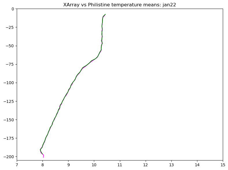
ax.plot( tmean_list, z, ms = 4., color='magenta')
ax.plot(r1['temperature'][0], r1['temperature'][0]['z'], color='green')
ax.set(ylim = (-205, 0), xlim = (7, 15), title='XArray vs Philistine temperature means: ' + month_choice)
[(-205.0, 0.0),
 (7.0, 15.0),
 Text(0.5, 1.0, 'XArray vs Philistine temperature means: jan22')]
# flag bug fix this for k in r1: print(k[0].name)
on to anomalies#
Now we have r1 which is reference for phase 1. Let’s generate both ascent and descent anomaly maps. Start with ascent.
r1 is a dictionary of 7 3-tuples keyed by an r1 sensor name from { conductivity, density, salinity, temperature, o2, chlora, bb, fdom }.
The 3-tuple is three DataArrays: (sensor, stddev, count)
n_profiles = len(profiles)
n_zbins    = n_zone_meters//n_meters_per_bin
anomalies  = {}
for sensor_name in sensors_phase1:

    a = np.zeros((n_zbins, n_profiles))     # bins are {-201 - -198, -198 - -195, ..., -3 - 0} qty 67
                                            #   So [-201, 198) -> 0, [-198, 195) -> 1... so rhs of bin 0 maps to integer 1
    for i in range(n_profiles):
        daData   = d[sensor_name][0].sel(time=slice(profiles["a0t"][i], profiles["a1t"][i]))
        daZ      = d[sensor_name][1].sel(time=slice(profiles["a0t"][i], profiles["a1t"][i]))
        zi_list  = [int((z + 201.)/3) for z in daZ]          # zi_list is: For each sample in a chosen profile: index of its z depth

        # list comprehension:
        #   j ranges across all of the indices for this particular profile (so a sample / time index)
        #   The calculated value for this j is (data - reference) / stddev where
        #       reference is the mean data value at this depth (indexed by zi_list[j])
        #       stddev is just that (indexed in the same manner)
        #       Note that data is referenced directly by the j index

        err_list = [(daData[j]-r1[sensor_name][0][zi_list[j]])/r1[sensor_name][1][zi_list[j]].data for j in range(len(zi_list))]
        for j in range(len(err_list)): a[zi_list[j], i] = err_list[j]
    anomalies[sensor_name] = a
    print('added ' + sensor_name + ' to anomaly dictionary')

    # the 100 depth cuts are -198, -196, ..., 0 so index by depth z is int((z + 198.)/2): 0, 1, ..., 99
    # ref value is r1['sensor_name'][0][j]
    # ref sd    is r1['sensor_name'][1][j]
added conductivity to anomaly dictionary
added density to anomaly dictionary
added salinity to anomaly dictionary
added temperature to anomaly dictionary
added do to anomaly dictionary
added chlora to anomaly dictionary
added bb to anomaly dictionary
added fdom to anomaly dictionary
for sensor in sensors_phase1:
    print(sensor, np.nanmean(anomalies[sensor]))
conductivity -0.08498533399890759
density 0.6648463740801844
salinity 0.3091199464205781
temperature -0.2125841424937772
do -0.2695350311676143
chlora -0.15013788633491132
bb 0.004646384676911033
fdom 0.08324104462216822
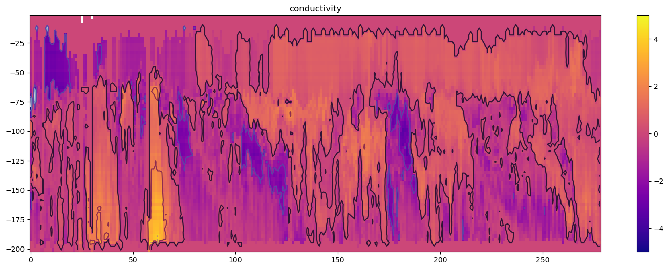
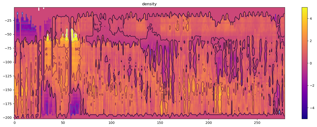
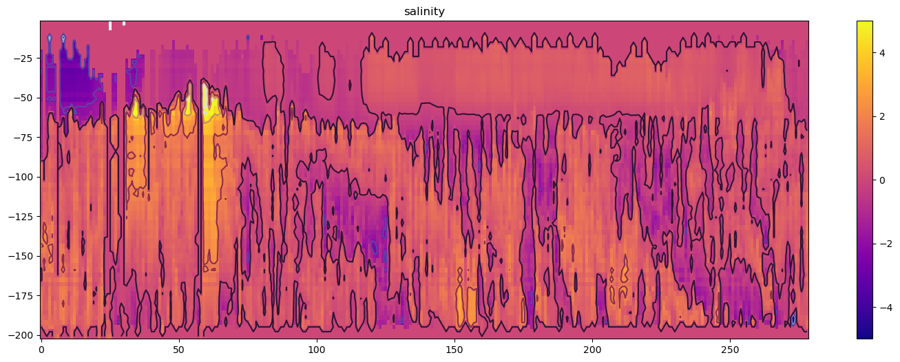
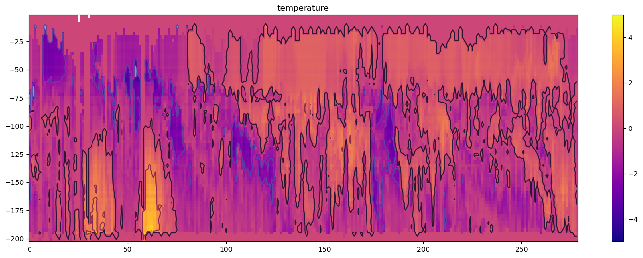
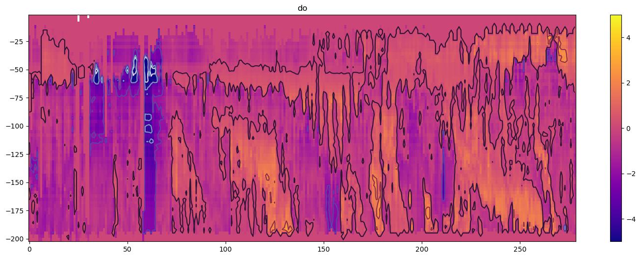
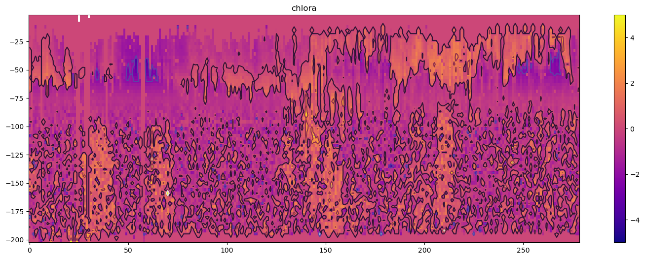
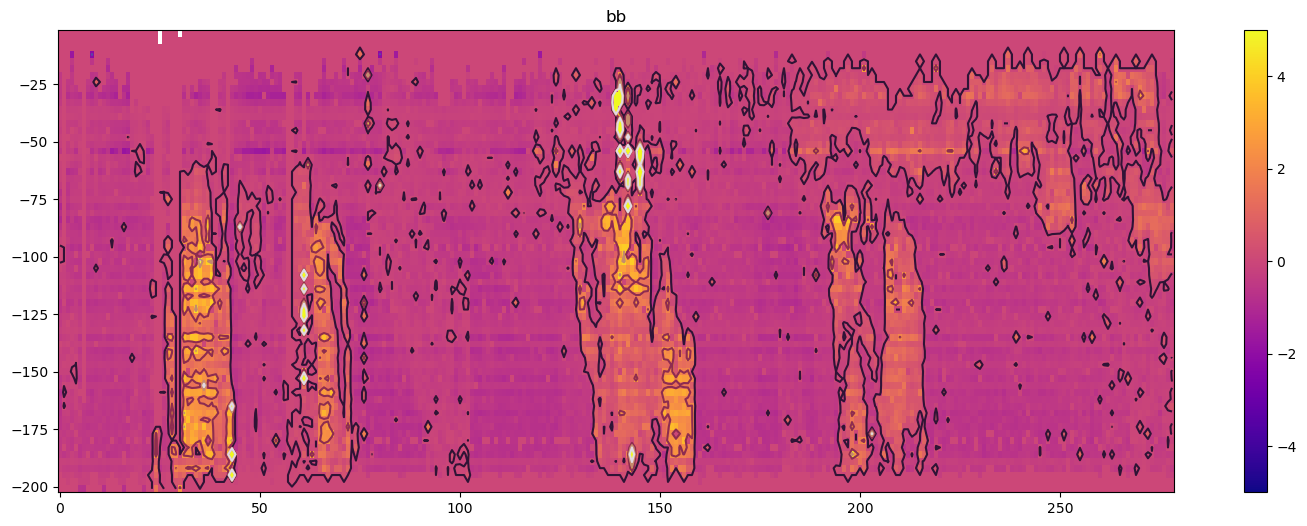
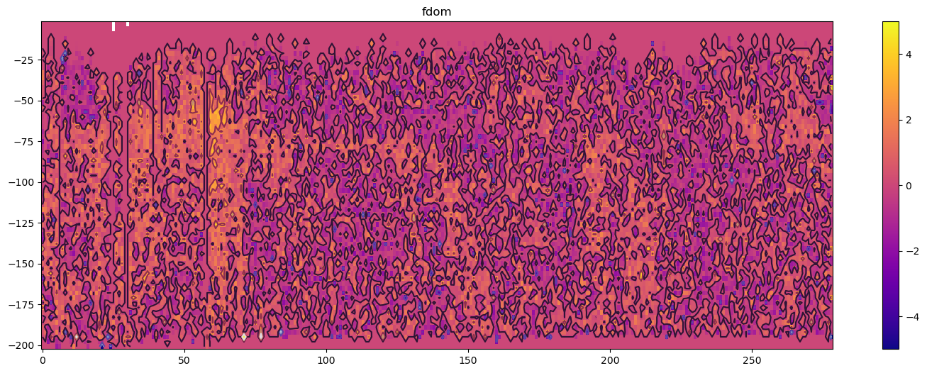
def PColorAndContour(sensor):
    x, y = np.arange(0, 279, 1.), np.arange(-201, 0, 3)
    X, Y = np.meshgrid(x, y)
    figure(figsize=(18, 6))
    plot = plt.pcolormesh(x, y, anomalies[sensor], cmap='plasma', vmin=-5, vmax=5)
    cset = plt.contour(X, Y, anomalies[sensor], [-6, -4, -2, 0, 2, 4, 6], cmap='twilight')      # plt.clabel(cset, inline=True)
    plt.colorbar(plot)
    plt.title(sensor)
    return 'hope this suits'

for sensor in sensors_phase1:
    PColorAndContour(sensor)
n_phase1 = len(sensors_phase1)

x, y = np.arange(0, 279, 1.), np.arange(-201, 0, 3)
X, Y = np.meshgrid(x, y)
im, ax_divider_list, colorbar_axis_list, colorbar_list = [], [], [], []

# fig, axs = plt.subplots(n_phase1, figsize=(16, 6*n_phase1))
# fig.subplots_adjust(wspace=0.5)

# my_plots = []

# for i in range(n_phase1):
#     sensor_name = sensors_phase1[i]
#     my_plots.append(axs[i].pcolormesh(X, Y, anomalies[sensor_name], cmap='gist_earth'))
#     axs[i].set(title=sensor_name)
#     my_plots[-1].colorbar()
fig, axs = plt.subplots(2, figsize=(16, 12))

for i in [0, 1]:
    im = axs[i].imshow(anomalies[sensors_phase1[i]], cmap='gist_earth')
    fig.colorbar(im, cax=axs[0], orientation='vertical')
    # plt.show()

    # just wrong: im.append(axs[i].imshow(anomalies[sensor_name]))
    # ax_divider_list.append(make_axes_locatable(im[i]))
    # cax.append(ax_divider[-1].append_axes("right", size="7%", pad="2%"))
    # cb.append(fig.colorbar(im[-1], cax=cax[-1]))


"""
plt.imshow(Bho, origin='l')
plt.contour(Bho, [300,400,500],origin='lower', colors=['white', 'yellow', 'red'])
plt.colorbar()
"""

plt.show()
# for this_ref in r1:
    # print(this_ref, ' has mean data array with name ' + r1[this_ref][0].name)