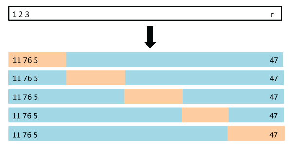
Cross-validation estimates how well a model generalizes by holding data out. The dataset is split into a training set and a validation set; the model learns on the first and is scored on the second. Repeating the split several times and averaging the scores gives a more reliable estimate than a single split, and lowers the risk of picking a model that just memorized the training data. See the scikit-learn tutorials on cross-validation.
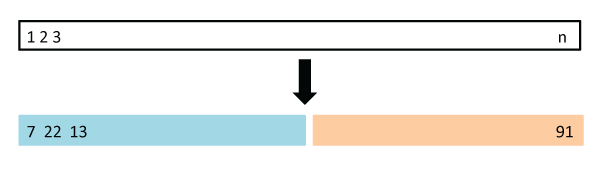 From scikit-learn: a single split into training and validation sets.
A single validation set is small, so its error estimate is noisy. Cross-validation over several folds averages the estimate over many held-out subsets:
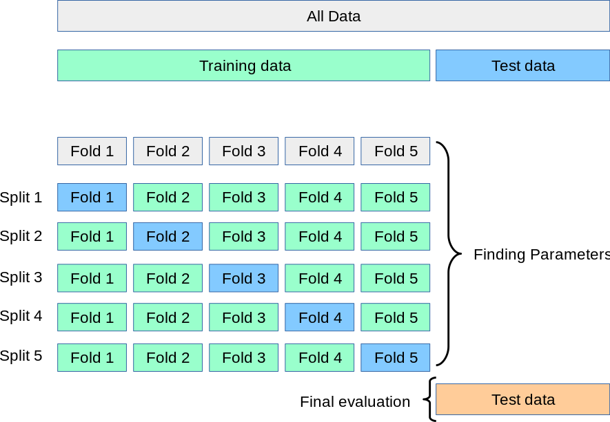 From scikit-learn.
In short, cross-validation serves three purposes: it estimates predictive performance on unseen data, it supports model selection and hyperparameter tuning, and it flags overfitting.
There is a catch, and it matters more in geoscience than almost anywhere else. Our data are correlated in time and space: a GNSS position today is nearly identical to yesterday’s, and a seismic station’s noise resembles its neighbor’s. When we shuffle correlated samples randomly into folds, every validation sample has near twins sitting in the training set. Information leaks from the validation set into training, and the scores lie. This lesson demonstrates the failure and the fix on a synthetic GNSS displacement series with known ground truth. Earlier editions of this book downloaded station P395 from the Nevada Geodetic Laboratory; the synthetic series keeps the same physics and adds ground truth we can check against. The second half of the lesson moves from time to space and groups: multi-site tables where the split must respect sites, clusters, and events.
1. A GNSS displacement series
The mlgeo_synth package generates a daily GNSS displacement series with known components: a secular velocity of 12 mm/yr, annual and semi-annual seasonal loading, a 25 mm coseismic step at day 1800 followed by logarithmic postseismic decay, and colored noise (white + flicker + random walk). The noise-free components come back as separate columns, so we can compare any estimate to the truth.
import matplotlib.pyplot as plt
import numpy as np
import pandas as pd
import mlgeo_synth
%matplotlib inline
g = mlgeo_synth.gnss_series(n_years=10.0, velocity_mm_yr=12.0, eq_day=1800, seed=42)
print(g.shape)
g.head()(3652, 5)
fig, axes = plt.subplots(2, 1, figsize=(10, 6), sharex=True)
axes[0].plot(g["date"], g["disp_mm"], lw=0.5, color="0.3")
axes[0].set_ylabel("displacement (mm)")
axes[0].set_title("Observed displacement (with colored noise)")
axes[1].plot(g["date"], g["trend_mm"], label="trend (12 mm/yr)")
axes[1].plot(g["date"], g["seasonal_mm"], label="seasonal")
axes[1].plot(g["date"], g["eq_mm"], label="coseismic + postseismic")
axes[1].set_ylabel("displacement (mm)")
axes[1].set_title("Noise-free components")
axes[1].legend(loc="upper left")
axes[1].set_xlabel("date")
plt.tight_layout()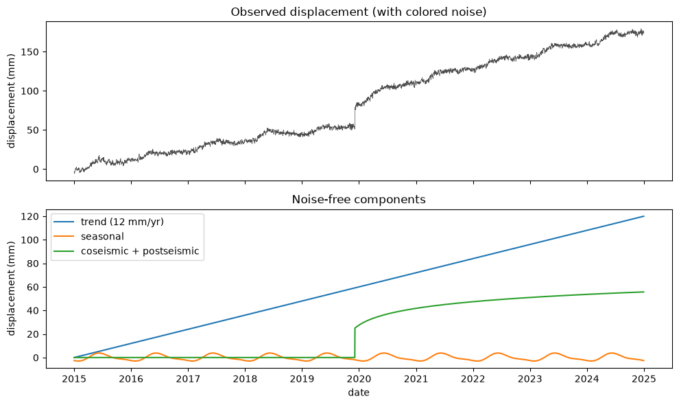
The observed series is the sum of the three components plus noise. The trend records plate motion. The seasonal term comes from hydrological and atmospheric loading. The earthquake term is a step plus a slow decay as the fault relaxes. The noise is not white: flicker and random-walk components make errors on nearby days strongly correlated, which is exactly what will break random cross-validation later.
Warm-up: fit the secular velocity. Before any cross-validation, fit a straight line to the whole series, as a geodesist would to estimate plate velocity.
from sklearn.linear_model import LinearRegression

t_years = ((g["date"] - g["date"].iloc[0]).dt.days / 365.25).to_numpy().reshape(-1, 1)
d = g["disp_mm"].to_numpy()

reg = LinearRegression()
reg.fit(t_years, d)
d_fit = reg.predict(t_years)

print(f"Fitted velocity: {reg.coef_[0]:.2f} mm/yr")
print("True velocity:   12.00 mm/yr")

plt.figure(figsize=(10, 3.5))
plt.plot(g["date"], d, lw=0.5, color="0.5", label="data")
plt.plot(g["date"], d_fit, color="C3", lw=2, label="linear fit")
plt.ylabel("displacement (mm)")
plt.legend()
plt.title("Linear velocity fit on the full series")
Fitted velocity: 19.52 mm/yr
True velocity: 12.00 mm/yr
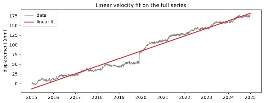
The fitted slope is off the true 12 mm/yr. The coseismic step and the postseismic decay push the line up, and the colored noise adds long-period wander that a straight line partly absorbs. A model can be simple, well fit, and still biased when the physics in the data is richer than the model.
2. A supervised forecasting task
Cross-validation questions get sharp when the model does something operational. Here is one: given the recent history of the station, where will it be next month? For each anchor day we build features from the last 60 days and predict the mean displacement over the next 30 days.
Features per anchor day:
- mean of the last 60 days
- mean of the last 10 days
- last observed value
- linear slope over the last 60 days (
np.polyfit) - sine and cosine of the day of year (to encode the season)
Target: mean displacement over the next 30 days.
We slide the anchor day forward with a stride of 5 days, which gives about 700 samples. Note what this construction does: neighboring anchor days share almost all of their window data. Sample i and sample i+1 overlap on 55 of 60 history days and 25 of 30 target days. The samples are strongly correlated by construction, just as they would be for any windowed geophysical time series.
disp = g["disp_mm"].to_numpy()
doy = g["date"].dt.dayofyear.to_numpy()

rows = []
for i in range(60, len(disp) - 30, 5):  # need 60 days history, 30 days future
    hist60 = disp[i - 60:i]
    rows.append({
        "mean_60d": hist60.mean(),
        "mean_10d": disp[i - 10:i].mean(),
        "last_val": disp[i - 1],
        "slope_60d": np.polyfit(np.arange(60), hist60, 1)[0],
        "doy_sin": np.sin(2 * np.pi * doy[i] / 365.25),
        "doy_cos": np.cos(2 * np.pi * doy[i] / 365.25),
        "target": disp[i:i + 30].mean(),
    })

feat = pd.DataFrame(rows)
X = feat.drop(columns="target").to_numpy()
y = feat["target"].to_numpy()
print(f"{len(feat)} samples, {X.shape[1]} features")
feat.head()
713 samples, 6 features
The model for every experiment below is the same random forest, so any difference in scores comes from the split, not the model.
from sklearn.ensemble import RandomForestRegressor

model = RandomForestRegressor(n_estimators=200, random_state=42)
3. The optimistic lie: random CV
First, the standard recipe most tutorials teach: shuffle the samples into 5 folds and score with cross_val_score. We try two shuffled schemes, KFold(shuffle=True) and ShuffleSplit, and report R² and mean absolute error.
from sklearn.model_selection import cross_val_score, KFold, ShuffleSplit

def cv_scores(model, X, y, cv, name):
    r2 = cross_val_score(model, X, y, cv=cv, scoring="r2")
    mae = -cross_val_score(model, X, y, cv=cv, scoring="neg_mean_absolute_error")
    print(f"{name:22s}  R2 = {r2.mean():6.3f} +/- {r2.std():.3f}   MAE = {mae.mean():5.2f} mm")
    return r2.mean(), mae.mean()

kf_shuffled = KFold(n_splits=5, shuffle=True, random_state=42)
ss = ShuffleSplit(n_splits=5, test_size=0.2, random_state=42)

results = {}
results["KFold (shuffled)"] = cv_scores(model, X, y, kf_shuffled, "KFold (shuffled)")
results["ShuffleSplit"] = cv_scores(model, X, y, ss, "ShuffleSplit")
KFold (shuffled) R2 = 1.000 +/- 0.000 MAE = 0.61 mm
ShuffleSplit R2 = 1.000 +/- 0.000 MAE = 0.58 mm
The scores look excellent: R² near 1, errors of a millimeter or two. If this were a paper, the model would be declared a success. It is not. The next section shows what the same model scores when the split respects time.
4. Honest splits for time series
TimeSeriesSplit trains on the past and validates on the future, which is how a forecast model is actually used. As an intermediate case we also try KFold without shuffling, which validates on contiguous blocks of time: no near duplicates across the boundary except at the block edges.
from sklearn.model_selection import TimeSeriesSplit

kf_blocks = KFold(n_splits=5, shuffle=False)
tss = TimeSeriesSplit(n_splits=5)

results["KFold (blocks)"] = cv_scores(model, X, y, kf_blocks, "KFold (blocks)")
results["TimeSeriesSplit"] = cv_scores(model, X, y, tss, "TimeSeriesSplit")

summary = pd.DataFrame(results, index=["mean R2", "mean MAE (mm)"]).T.round(3)
summary
KFold (blocks) R2 = -1.728 +/- 2.126 MAE = 11.54 mm
TimeSeriesSplit R2 = -4.267 +/- 3.704 MAE = 16.44 mm
Same model, same data, and the honest schemes report far worse skill. To see why, plot which samples land in training and which in validation for each scheme. Sample index runs left to right, which here is also time.
schemes = {"ShuffleSplit": ss, "KFold (shuffled)": kf_shuffled, "TimeSeriesSplit": tss}

fig, axes = plt.subplots(3, 1, figsize=(10, 7), sharex=True)
for ax, (name, cv) in zip(axes, schemes.items()):
    for fold, (tr_idx, va_idx) in enumerate(cv.split(X)):
        ax.scatter(tr_idx, np.full(len(tr_idx), fold), marker="|", s=60,
                   color="C0", label="train" if fold == 0 else None)
        ax.scatter(va_idx, np.full(len(va_idx), fold), marker="|", s=60,
                   color="C1", label="validation" if fold == 0 else None)
    ax.set_yticks(range(5))
    ax.set_ylabel("fold")
    ax.set_title(name)
    ax.legend(loc="center left", bbox_to_anchor=(1.0, 0.5))
axes[-1].set_xlabel("sample index (time order)")
plt.tight_layout()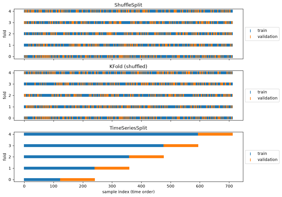
In the two shuffled panels, orange validation samples are sprinkled among blue training samples. Every validation sample has immediate neighbors in the training set, and those neighbors share 55 of its 60 history days. The forest does not need to forecast anything; it interpolates its neighbors, and the score measures memorization. TimeSeriesSplit (bottom panel) always validates on data later than everything trained on. The model must extrapolate into a future it has never seen, and the score reflects the skill it would have in deployment.
Contiguous blocks (KFold without shuffling) sit in between: leakage only happens near the block edges, so the scores drop most of the way toward the honest number. Blocked splits are the right idea whenever there is no single time axis, for example spatial blocks of stations.
5. Every score needs a baseline and an error bar
The honest scores in Section 4 look bad. How bad? Two habits put any score in context: compare it to a baseline that requires no learning, and put an error bar on it.
The natural baseline for a forecast is persistence: the future looks like the present. Here the persistence forecast of the next-30-day mean is just the last observed value, a feature we already computed (last_val). It costs nothing and encodes the strongest property of the series: it changes slowly.
from sklearn.metrics import mean_absolute_error, r2_score

persist = feat["last_val"].to_numpy()
rows_bl = []
abs_err = []  # per-sample validation errors in time order, for the bootstrap below
for fold, (tr, va) in enumerate(tss.split(X)):
    fitted = RandomForestRegressor(n_estimators=200, random_state=42).fit(X[tr], y[tr])
    pred = fitted.predict(X[va])
    abs_err.append(np.abs(y[va] - pred))
    rows_bl.append({
        "model MAE (mm)": mean_absolute_error(y[va], pred),
        "persistence MAE (mm)": mean_absolute_error(y[va], persist[va]),
        "model R2": r2_score(y[va], pred),
        "persistence R2": r2_score(y[va], persist[va]),
    })
abs_err = np.concatenate(abs_err)
pd.DataFrame(rows_bl).rename_axis("fold").round(2)The comparison is humbling. Persistence forecasts the 30-day mean to within about 2 mm and scores R² near 0.9 on every fold; the forest is an order of magnitude worse. The reason is extrapolation: the station keeps moving at 12 mm/yr, so every validation target sits above the range of targets the forest trained on, and a forest cannot predict outside the range of its training labels. Persistence rides the trend for free.
Note the model’s negative R² values. R² compares a model against the constant that predicts the mean of the validation targets, so R² < 0 means the model is worse than predicting the mean — no skill at all. Whenever a paper reports forecast skill without a persistence (or climatology) baseline, ask what the baseline would have scored.
The error bar. A single number like “MAE = 16 mm” hides how uncertain the estimate itself is. The bootstrap puts an interval on it: resample the validation errors with replacement, recompute the MAE of each resample, and read a confidence interval from the spread. For independent errors, resampling single errors (the simple bootstrap) is enough. Our errors are autocorrelated — neighboring anchor days share most of their window — so single-error resampling pretends there is more independent information than there is, and the interval comes out too narrow. The moving-block bootstrap resamples contiguous blocks (here 12 samples, or 60 days at the 5-day stride), so each resample keeps the local correlation.
rng = np.random.default_rng(0)
n = len(abs_err)
n_boot = 2000

# simple bootstrap: resample individual errors
simple = np.array([rng.choice(abs_err, n).mean() for _ in range(n_boot)])

# moving-block bootstrap: resample contiguous blocks of 12 samples (60 days)
L = 12
n_blocks = int(np.ceil(n / L))
starts = rng.integers(0, n - L + 1, size=(n_boot, n_blocks))
block = np.array([
    np.concatenate([abs_err[s:s + L] for s in row])[:n].mean() for row in starts
])

print(f"pooled honest MAE: {abs_err.mean():.1f} mm")
print(f"simple bootstrap 95% CI:       "
      f"[{np.percentile(simple, 2.5):.1f}, {np.percentile(simple, 97.5):.1f}] mm")
print(f"moving-block bootstrap 95% CI: "
      f"[{np.percentile(block, 2.5):.1f}, {np.percentile(block, 97.5):.1f}] mm")
pooled honest MAE: 16.4 mm
simple bootstrap 95% CI: [15.5, 17.5] mm
moving-block bootstrap 95% CI: [13.2, 20.1] mm
The block interval is about twice as wide as the simple one. Same data, same statistic; the only difference is the independence assumption. Correlated errors carry fewer effective samples than their count suggests, and the simple bootstrap’s narrow interval is one more form of the optimism this whole lesson is about. Report the interval that matches the correlation structure of the errors, and report it next to the point estimate.
6. Leave-One-Out CV
LOOCV splits the data into training and validation sets n times, where n is the number of data points. Each round, the training set is all but one sample and the validation set is that single held-out sample.
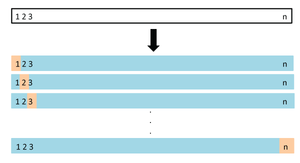
Advantages: low bias with respect to the training data, and the result is deterministic, since there is no random split to repeat. Disadvantage: it costs n model fits, which is expensive for anything but small datasets and cheap models.
We demonstrate on the simple velocity-regression problem, subsampled to every 20th day so the n fits stay fast.
from sklearn.model_selection import LeaveOneOut
from sklearn.metrics import mean_squared_error

t_sub = t_years[::20]           # ~180 points
d_sub = d[::20]
print(f"{len(d_sub)} points -> {len(d_sub)} fits")

loo = LeaveOneOut()
vels, mse_val = [], []
for train_idx, val_idx in loo.split(t_sub):
    t_train, t_val = t_sub[train_idx], t_sub[val_idx]
    d_train, d_val = d_sub[train_idx], d_sub[val_idx]
    reg = LinearRegression().fit(t_train, d_train)
    vels.append(reg.coef_[0])
    mse_val.append(mean_squared_error(d_val, reg.predict(t_val)))

vels, mse_val = np.array(vels), np.array(mse_val)
print(f"Velocity estimates: mean {vels.mean():.3f} mm/yr, std {vels.std():.4f} mm/yr")
print(f"Mean validation MSE: {mse_val.mean():.2f} mm^2")
183 points -> 183 fits
Velocity estimates: mean 19.427 mm/yr, std 0.0146 mm/yr
Mean validation MSE: 106.93 mm^2
The velocity barely moves when one point is dropped, so the spread across the n fits is tiny. Two cautions. First, LOOCV is rarely worth the cost: n fits for an error estimate that k-fold approximates with 5 or 10. Second, LOOCV does not fix correlation. Each held-out point’s immediate neighbors are always in the training set, so for an autocorrelated series LOOCV is close to the most optimistic split possible: it is the shuffled-fold problem taken to its limit.
7. Hyperparameter search under honest CV
Models have parameters learned from the data (tree splits, regression weights) and hyperparameters set before training (tree depth, leaf size). Hyperparameter tuning searches for the settings that score best under cross-validation, and it is standard practice. The usual approaches:
- Manual tuning: adjust by hand, guided by knowledge of the problem. Good for building intuition; not systematic.
- Grid search: evaluate every combination in a predefined grid. Thorough but expensive as the grid grows. In scikit-learn:
GridSearchCV. - Random search: draw combinations from predefined distributions for a fixed budget of iterations. Covers wide spaces more cheaply than a grid. In scikit-learn:
RandomizedSearchCV. - Bayesian optimization: model the score as a function of the hyperparameters and spend evaluations where improvement looks likely (e.g.
optuna,scikit-optimize).
The choice of CV scheme inside the search matters as much as the search itself. Tuning against shuffled folds selects the model that best memorizes its neighbors. We tune against TimeSeriesSplit, so the winner is the best forecaster.
from sklearn.model_selection import GridSearchCV

param_grid = {"max_depth": [2, 4, 8, None], "min_samples_leaf": [1, 5, 20]}

grid = GridSearchCV(
    RandomForestRegressor(n_estimators=100, random_state=42),
    param_grid,
    cv=TimeSeriesSplit(n_splits=5),
    scoring="neg_mean_absolute_error",
)
grid.fit(X, y)
print("Best params:", grid.best_params_)
print(f"Best CV MAE: {-grid.best_score_:.2f} mm")
Best params: {'max_depth': 4, 'min_samples_leaf': 5}
Best CV MAE: 15.90 mm
For random search, pass the frozen scipy.stats distribution objects. An earlier version of this notebook pre-sampled with randint.rvs(size=10), which collapses random search onto a fixed list of ten values; passing the frozen distribution lets every iteration draw fresh values.
from sklearn.model_selection import RandomizedSearchCV
from scipy.stats import randint

distributions = {"max_depth": randint(1, 10), "min_samples_leaf": randint(1, 10)}

rand = RandomizedSearchCV(
    RandomForestRegressor(n_estimators=100, random_state=42),
    distributions,
    n_iter=15,
    random_state=0,
    cv=TimeSeriesSplit(n_splits=5),
    scoring="neg_mean_absolute_error",
)
rand.fit(X, y)
print("Best params:", rand.best_params_)
print(f"Best CV MAE: {-rand.best_score_:.2f} mm")
print(f"Grid search best MAE was {-grid.best_score_:.2f} mm")
Best params: {'max_depth': 9, 'min_samples_leaf': 5}
Best CV MAE: 15.98 mm
Grid search best MAE was 15.90 mm
The two searches land within a fraction of a millimeter of each other: with only two hyperparameters, 15 random draws probe the space about as well as a 12-point grid, and random search scales better when the space grows.
8. Space and groups: the same lie on a map
Time is not the only axis along which geoscience data are correlated. Field campaigns produce grouped data: several soundings at each site, several sites along each road or basin, and a target that rides on a smooth regional field. Two observations from the same site are near copies; two sites in the same cluster are close cousins.
mlgeo_synth.multisite_table builds that geometry with ground truth: 6 clusters of 5 sites each, 10 repeat observations per site (300 rows). The target is a linear signal in the feat_* columns — the transportable part of the skill — plus a smooth regional field (correlation length 25 km) evaluated at each site, plus noise. The field is returned as a callable in truth, so we can draw the map the model is secretly memorizing.
from sklearn.model_selection import GroupKFold, StratifiedGroupKFold

sites, truth = mlgeo_synth.multisite_table(seed=13)
print(sites.shape)
sites.head()
(300, 8)
gx = np.linspace(-5, 105, 220)
GX, GY = np.meshgrid(gx, gx)
F = truth["field"](GX.ravel(), GY.ravel()).reshape(GX.shape)

fig, ax = plt.subplots(figsize=(7.5, 6))
im = ax.pcolormesh(GX, GY, F, cmap="viridis", shading="auto")
fig.colorbar(im, ax=ax, label="regional field (target units)")
site_locs = sites.drop_duplicates("site_id")
for cl, grp in site_locs.groupby("cluster_id"):
    ax.scatter(grp["x_km"], grp["y_km"], s=50, edgecolor="white",
               linewidth=1.2, label=f"cluster {cl}")
ax.set_xlabel("x (km)")
ax.set_ylabel("y (km)")
ax.set_title("Regional field with clustered sites (10 observations per site)")
ax.legend(loc="upper center", bbox_to_anchor=(0.5, -0.12), ncols=6, title=None)
plt.tight_layout()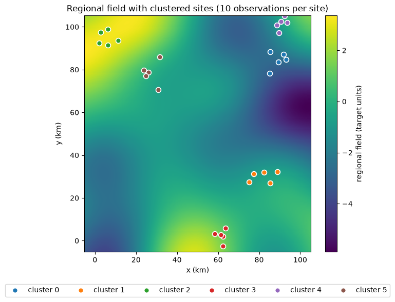
The map is the mechanism. The field varies smoothly over ~25 km, and the sites sit in tight clusters a few km across, so every site in a cluster shares nearly the same field value — and all 10 observations of a site share it exactly. A shuffled split hands the model those near copies.
Now the split ladder. Same forest, same data, three splits that hold out progressively more of the shared structure: shuffled KFold, GroupKFold on site_id (whole sites held out), and GroupKFold on cluster_id with 6 splits — leave-one-cluster-out, the discrete version of a blocked spatial split. We run the ladder twice: once on the feat_* columns alone, and once adding the coordinates x_km, y_km as features.
feat_cols = [c for c in sites.columns if c.startswith("feat_")]
y_site = sites["target"].to_numpy()

ladder = {
    "KFold (shuffled)": (KFold(n_splits=5, shuffle=True, random_state=42), None),
    "GroupKFold (site)": (GroupKFold(n_splits=5), sites["site_id"]),
    "GroupKFold (cluster)": (GroupKFold(n_splits=6), sites["cluster_id"]),
}

rows_ladder = []
for feats_name, cols in [("features only", feat_cols),
                         ("features + x,y", feat_cols + ["x_km", "y_km"])]:
    X_site = sites[cols].to_numpy()
    for rung, (cv, groups) in ladder.items():
        r2 = cross_val_score(model, X_site, y_site, cv=cv, groups=groups, scoring="r2")
        rows_ladder.append({"features": feats_name, "split": rung,
                            "mean R2": r2.mean(), "std R2": r2.std()})
pd.DataFrame(rows_ladder).round(3)Read the ladder top to bottom; each rung asks a harder, and more honest, question.
- KFold (shuffled), R² ≈ 0.7. Every held-out observation has up to 9 siblings from its own site in training. The forest recognizes the site from its features and recalls that site’s field value. The score answers: “how well can I predict another sounding at a site I already surveyed?”
- GroupKFold by site, R² ≈ 0.35. Whole sites are held out, so site memorization is gone — but held-out sites still have cluster neighbors in training that share the field. The score answers: “a new site inside a surveyed cluster?”
- Leave-cluster-out, R² < 0. Whole clusters are held out and the model faces a region it has never seen. The field value there is unknowable from the training data, and the forest’s memorized field offsets actively mislead it — worse than predicting the mean (Section 5). The score answers the question a regional hazard map actually poses: “a new region?”
Adding x_km, y_km sharpens the contrast. Under shuffled CV the forest now interpolates the map almost perfectly (R² ≈ 0.95) — a genuinely useful skill within the surveyed region. Under leave-cluster-out the same coordinates make things worse: they point to parts of the map the training data never constrained. Same model, same features, opposite verdicts — because interpolation between surveyed sites and extrapolation to a new region are different claims, and the split decides which claim the score supports. In continuous settings without natural clusters, the same idea becomes a buffered spatial split: exclude from training everything within a correlation length of the validation sites.
Notebook 4.5 (Section 4.6) crosses this line deliberately: a deep ensemble trained on a bounded compositional range is evaluated out of range — including the one error its disagreement fails to flag.
9. Small, clustered, imbalanced: when grouped CV itself breaks
Grouped data in geotechnical and geological practice is usually also small and imbalanced: a few hundred case histories, a rare positive class (liquefaction observed, landslide occurred, mineralization present), and positives that cluster in space because the driving field does. That combination is the norm, not the corner case, wherever labels come from case histories rather than surveys. multisite_table(binary=True) reproduces it: the same 300-row site geometry, with the latent target thresholded so 12% of rows are positive.
Grouping by site is still mandatory — but now it can fail on its own terms. GroupKFold deals out whole sites without looking at labels, and because positives are spatially clustered, a fold can end up with no positives at all. ROC AUC is undefined on a fold with one class.
import warnings
from sklearn.ensemble import RandomForestClassifier

cases, truth_b = mlgeo_synth.multisite_table(binary=True, seed=1)
X_case = cases[feat_cols].to_numpy()
y_case = cases["label"].to_numpy()
print(f"{y_case.sum()} positives in {len(y_case)} rows ({y_case.mean():.0%})")

clf = RandomForestClassifier(n_estimators=200, random_state=42)
gkf = GroupKFold(n_splits=5)

pos_per_fold = [int(y_case[va].sum())
                for _, va in gkf.split(X_case, y_case, groups=cases["site_id"])]
print("positives per validation fold:", pos_per_fold)

with warnings.catch_warnings():
    warnings.simplefilter("ignore")  # sklearn warns about the undefined fold
    auc_gkf = cross_val_score(clf, X_case, y_case, cv=gkf,
                              groups=cases["site_id"], scoring="roc_auc")
print("GroupKFold AUC per fold:", np.round(auc_gkf, 3))
36 positives in 300 rows (12%)
positives per validation fold: [11, 5, 0, 18, 2]
GroupKFold AUC per fold: [0.834 0.98 nan 0.997 0.754]
The nan is not a scikit-learn bug; it is the data reporting that this grouped split left one fold with zero positives, so there is no ROC curve to compute — and averaging the remaining folds quietly changes what the mean estimates. The repair is StratifiedGroupKFold: keep every site intact and balance the positive fraction across folds.
sgkf = StratifiedGroupKFold(n_splits=5, shuffle=True, random_state=0)
pos_sgkf = [int(y_case[va].sum())
            for _, va in sgkf.split(X_case, y_case, groups=cases["site_id"])]
print("positives per validation fold:", pos_sgkf)

auc_sgkf = cross_val_score(clf, X_case, y_case, cv=sgkf,
                           groups=cases["site_id"], scoring="roc_auc")
print(f"StratifiedGroupKFold AUC = {auc_sgkf.mean():.3f} +/- {auc_sgkf.std():.3f}")
positives per validation fold: [8, 7, 7, 4, 10]
StratifiedGroupKFold AUC = 0.925 +/- 0.025
Every fold now has positives and every fold returns a number. Keep the fold-to-fold spread in the report: with 36 positives split five ways, each fold’s AUC rests on a handful of events, and the spread (or a bootstrap interval, Section 5) is as informative as the mean.
10. Grouping by event: aftershocks and quarry blasts
In seismology the group is usually the event. mlgeo_synth.event_station_table builds a toy ground-motion dataset: 60 earthquakes in 4 clusters (compact in space and time, like mainshock–aftershock sequences), each recorded by the same 15 stations — 900 recordings. Log peak ground acceleration follows a toy attenuation relation in magnitude and distance, plus a per-event term shared by all 15 recordings of an event and a per-station term. The event term is the leakage: a random split puts 12 recordings of an event in training and 3 in validation, and the model gets credit for recalling that event’s offset.
gm, truth_gm = mlgeo_synth.event_station_table(seed=0)
X_gm = gm[["magnitude", "dist_km"]].to_numpy()
y_gm = gm["log10_pga"].to_numpy()

r2_rand = cross_val_score(model, X_gm, y_gm,
                          cv=KFold(n_splits=5, shuffle=True, random_state=42), scoring="r2")
r2_event = cross_val_score(model, X_gm, y_gm, cv=GroupKFold(n_splits=5),
                           groups=gm["event_id"], scoring="r2")
print(f"KFold (shuffled):      R2 = {r2_rand.mean():.3f} +/- {r2_rand.std():.3f}")
print(f"GroupKFold (event_id): R2 = {r2_event.mean():.3f} +/- {r2_event.std():.3f}")
KFold (shuffled): R2 = 0.845 +/- 0.014
GroupKFold (event_id): R2 = 0.600 +/- 0.150
Grouping by event costs about a quarter of the apparent skill, and the grouped number is the one that predicts performance on the next earthquake. The classification version of this trap is common: hundreds of aftershocks of one mainshock, or repeated blasts from one quarry, are near copies of each other, and a random split lets a classifier score high by recognizing the source rather than the source type. That is exactly the leakage the boxed admonition in 3.5 declares and tolerates — the leaderboard feature tables carry no event ID to group by. Here the metadata exists, so the cost of that concession is measurable: it is the gap between the two rows above.
11. Choosing the split
Every scheme in this lesson answers the same question posed at a different scale of shared structure. Before trusting any score, ask: what structure does my data share that the split must respect — time, site, event, or space? Observations sharing a window of time call for TimeSeriesSplit or contiguous blocks; sharing a site or instrument, GroupKFold by site; sharing a source event, GroupKFold by event; sharing a region, leave-cluster-out or a buffered spatial split. The leakage audit of 2.13 asks this question before training; the split choice is the same audit applied to evaluation. And when the metadata needed to group by is missing, say so and state what the score can and cannot mean, as the 3.5 leaderboard admonition does.