In this notebook we classify seismic recordings into four source types — earthquake, explosion, surface event, and noise — from 61 physical waveform features (spectral shape, envelope statistics, kurtosis, band energies). The dataset is a curated set of Pacific Northwest seismic events, 1000 per class, archived on Zenodo: DOI 10.5281/zenodo.14025693.
We compare three classic classifiers: Support Vector Machine, k-nearest neighbors, and Random Forest, and we evaluate them per class with classification reports, confusion matrices, and one-vs-rest ROC curves.
This dataset returns in notebook 3.9, and it anchors the class leaderboard defined at the end of this notebook.
1. Load the data
The loader below downloads and caches the four class files, concatenates them into one table, and drops the one feature column with missing values.
import numpy as np
import pandas as pd
import matplotlib.pyplot as plt
import pooch
SEISMIC_FILES = {
"1000_earthquakes_physical_features.csv": "md5:28129c8dd1b3e14f655d489577b841b5",
"1000_explosion_physical_features.csv": "md5:af1342d32e163e961e043364136359b0",
"1000_noise_physical_features.csv": "md5:16cdb992fed6cf6273d5624f5df905da",
"1000_surface_physical_features.csv": "md5:9a2c2643030cf058704d68e130654e9d",
}
frames = []
for fname, checksum in SEISMIC_FILES.items():
path = pooch.retrieve(
url=f"https://zenodo.org/api/records/14025693/files/{fname}/content",
known_hash=checksum,
fname=fname,
path=pooch.os_cache("mlgeo"),
)
frames.append(pd.read_csv(path, index_col=0))
seismic = pd.concat(frames, ignore_index=True)
seismic = seismic.dropna(axis=1) # drops the one feature column with missing values2. Explore
Check the class balance first. The four classes have 1000 events each, so this curated set is balanced. Keep in mind that real catalogs are not.
seismic["source"].value_counts().plot(kind="bar")
plt.ylabel("Number of events")
plt.title("Class balance")
plt.tight_layout()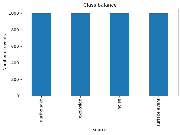
Build the feature matrix X (61 numeric waveform features) and the label vector y (four source-type strings).
X = seismic.drop(columns=["source", "serial_no"])
y = seismic["source"]
print("X:", X.shape, " y:", y.shape)
print("A few feature names:", list(X.columns[:8]))
X: (4000, 61) y: (4000,)
A few feature names: ['Window_Length', 'RappMaxMean', 'RappMaxMedian', 'AsDec', 'KurtoSig', 'KurtoEnv', 'SkewSig', 'SkewEnv']
3. Train/test split
The cell below is the canonical split for this chapter: this exact line defines the leaderboard split at the end of the notebook. Everyone trains on the same X_train and predicts on the same X_test.
Two details matter:
- An earlier version of this lesson used
shuffle=False. With the table ordered by class, that put whole classes in the test set and none in training — the classifier never saw the classes it was scored on. stratify=ypreserves the class proportions in both halves. That matters most when classes are imbalanced, and real seismic catalogs are: noise windows outnumber earthquakes by orders of magnitude.
from sklearn.model_selection import train_test_split
X_train, X_test, y_train, y_test = train_test_split(X, y, test_size=0.25, random_state=2026, stratify=y)4. Scale after the split
We fit the scaler on the training set only, then transform both sets. Fitting the scaler on all the data would let the test set’s statistics leak into training.
from sklearn.preprocessing import StandardScaler
scaler = StandardScaler()
X_train_scaled = scaler.fit_transform(X_train)
X_test_scaled = scaler.transform(X_test)
5. Baseline
Before any model, score a trivial baseline. DummyClassifier(strategy="most_frequent") always predicts the majority class; with four balanced classes it scores 0.25. Every model below must beat this number.
from sklearn.dummy import DummyClassifier
from sklearn import metrics

dummy = DummyClassifier(strategy="most_frequent")
dummy.fit(X_train, y_train)
baseline_acc = metrics.accuracy_score(y_test, dummy.predict(X_test))
print("Baseline accuracy:", baseline_acc)
Baseline accuracy: 0.25
6. Three classifiers
The SVM and k-nearest neighbors both rely on distances or margins in feature space, so they use the scaled features.
from sklearn.svm import SVC
from sklearn.neighbors import KNeighborsClassifier
from sklearn.ensemble import RandomForestClassifier

# Support Vector Machine classifier
clf = SVC(gamma='scale')  # model design
clf.fit(X_train_scaled, y_train)  # learn
svc_prediction = clf.predict(X_test_scaled)  # predict on test
print("SVC test accuracy:", metrics.accuracy_score(y_true=y_test, y_pred=svc_prediction))

# K-nearest Neighbors
knn_clf = KNeighborsClassifier()  # model design
knn_clf.fit(X_train_scaled, y_train)  # learn
knn_prediction = knn_clf.predict(X_test_scaled)  # predict on test
print("K-nearest Neighbors test accuracy:", metrics.accuracy_score(y_true=y_test, y_pred=knn_prediction))
SVC test accuracy: 0.877
K-nearest Neighbors test accuracy: 0.83
Random Forest works on the unscaled features: trees split on thresholds, and a monotonic rescaling does not change which side of a threshold a point falls on.
# Random Forest, on the unscaled features
rf_clf = RandomForestClassifier(random_state=42)  # model design
rf_clf.fit(X_train, y_train)  # learn
rf_prediction = rf_clf.predict(X_test)  # predict on test
print("Random Forest test accuracy:", metrics.accuracy_score(y_true=y_test, y_pred=rf_prediction))
Random Forest test accuracy: 0.882
7. Per-class evaluation
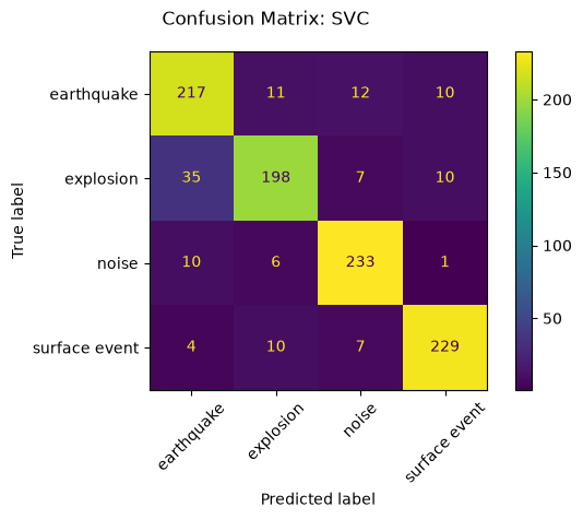
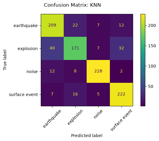
Accuracy is one number. The classification report gives precision, recall, and F1 per class, and the confusion matrix shows which classes get mistaken for each other.
from sklearn.metrics import ConfusionMatrixDisplay

print("Support Vector Machine")
print(f"Classification report for classifier {clf}:\n"
      f"{metrics.classification_report(y_test, svc_prediction)}\n")

disp = ConfusionMatrixDisplay.from_estimator(clf, X_test_scaled, y_test, xticks_rotation=45)
disp.figure_.suptitle("Confusion Matrix: SVC")
plt.tight_layout()
plt.show()
Support Vector Machine
Classification report for classifier SVC():
precision recall f1-score support
earthquake 0.82 0.87 0.84 250
explosion 0.88 0.79 0.83 250
noise 0.90 0.93 0.92 250
surface event 0.92 0.92 0.92 250
accuracy 0.88 1000
macro avg 0.88 0.88 0.88 1000
weighted avg 0.88 0.88 0.88 1000
print("K-nearest neighbors")
print(f"Classification report for classifier {knn_clf}:\n"
      f"{metrics.classification_report(y_test, knn_prediction)}\n")

disp = ConfusionMatrixDisplay.from_estimator(knn_clf, X_test_scaled, y_test, xticks_rotation=45)
disp.figure_.suptitle("Confusion Matrix: KNN")
plt.tight_layout()
plt.show()
K-nearest neighbors
Classification report for classifier KNeighborsClassifier():
precision recall f1-score support
earthquake 0.78 0.84 0.81 250
explosion 0.79 0.68 0.73 250
noise 0.92 0.91 0.92 250
surface event 0.83 0.89 0.86 250
accuracy 0.83 1000
macro avg 0.83 0.83 0.83 1000
weighted avg 0.83 0.83 0.83 1000
print("Random Forest")
print(f"Classification report for classifier {rf_clf}:\n"
      f"{metrics.classification_report(y_test, rf_prediction)}\n")

disp = ConfusionMatrixDisplay.from_estimator(rf_clf, X_test, y_test, xticks_rotation=45)
disp.figure_.suptitle("Confusion Matrix: Random Forest")
plt.tight_layout()
plt.show()
Random Forest
Classification report for classifier RandomForestClassifier(random_state=42):
precision recall f1-score support
earthquake 0.83 0.86 0.85 250
explosion 0.87 0.80 0.83 250
noise 0.93 0.94 0.93 250
surface event 0.90 0.94 0.92 250
accuracy 0.88 1000
macro avg 0.88 0.88 0.88 1000
weighted avg 0.88 0.88 0.88 1000
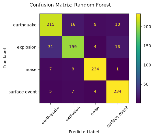
Which class pairs get confused the most? Compare the off-diagonal terms across the three confusion matrices. A cross-tabulation of true labels against Random Forest predictions makes the counts easy to read.
pd.crosstab(y_test, rf_prediction, rownames=["true"], colnames=["predicted"])The dominant confusion is between explosions and earthquakes. That is physically plausible: quarry blasts and shallow earthquakes excite similar frequency content at regional distances, so their waveform features overlap.
8. One-vs-rest ROC curves
ROC curves are defined for binary problems. For a multiclass problem we use the one-vs-rest strategy: binarize the labels (one column per class) and fit one binary classifier per class.
To keep the split identical to the canonical one, we binarize y_train and y_test obtained above rather than re-splitting the data.
from sklearn.multiclass import OneVsRestClassifier
from sklearn.preprocessing import label_binarize
from sklearn import svm
from sklearn.metrics import roc_curve, auc

classes = ['earthquake', 'explosion', 'noise', 'surface event']
y_train_bin = label_binarize(y_train, classes=classes)
y_test_bin = label_binarize(y_test, classes=classes)

ovr_classifier = OneVsRestClassifier(svm.SVC(kernel='linear'))
y_score = ovr_classifier.fit(X_train_scaled, y_train_bin).decision_function(X_test_scaled)

plt.figure(figsize=(7, 6))
plt.plot([0, 1], [0, 1], 'k--', label='chance')
for i, name in enumerate(classes):
    fpr, tpr, _ = roc_curve(y_test_bin[:, i], y_score[:, i])
    plt.plot(fpr, tpr, label=f'{name} (AUC = {auc(fpr, tpr):.2f})')
plt.xlim([0.0, 1.0])
plt.ylim([0.0, 1.05])
plt.grid(True)
plt.xlabel('False Positive Rate')
plt.ylabel('True Positive Rate')
plt.title('One-vs-rest ROC curves, linear SVC')
plt.legend(loc="lower right")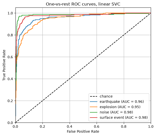
Class leaderboard
Train any classifier you like on X_train. Feature engineering is allowed. Do not peek at y_test while developing: select your model and hyperparameters with cross-validation on the training set only — scoring candidates on rotating validation subsets carved from the training data (lesson 3.8).
When you are done:
- Predict on the canonical
X_test(the split cell in section 3 defines it). - Save your predictions to
results/predictions_<uwnetid>.csvwith the format below. - Submit the file by pull request to the course repository. CI scores macro-F1 — the per-class F1 scores averaged with equal weight on every class — against the held-out labels and posts a leaderboard.
The row_id column is the row position in the canonical concatenated table; the split preserves it, so it identifies each test sample. The demo below writes a submission file from the Random Forest predictions.
import os
os.makedirs("results", exist_ok=True)
pred_df = pd.DataFrame({"row_id": X_test.index, "prediction": rf_prediction})
pred_df.to_csv("results/predictions_example.csv", index=False)
pred_df.head()- Kharita, A. (2024). Physical features for small sample of data (1000 events per class). Zenodo. 10.5281/ZENODO.14025693