3.9 Ensemble learning - Machine Learning in the Geosciences

Ensemble learning combines several weak learners into a strong learner that is more robust and generalizes better. A familiar example is the Random Forest, which is much stronger than the individual decision trees that compose it.

Key advantages of ensemble learning:

Reduced overfitting: bagging methods like Random Forests reduce the risk of overfitting by combining predictions from multiple models.
Improved generalization: combined models capture complex relationships more effectively and generalize better on diverse data.
Robustness to noise and outliers: aggregating predictions over many models dilutes the influence of individual noisy or outlier-laden data points.
Increased stability: individual models might do well on some subsets of the data and poorly on others; combining diverse models gives more stable predictions across subgroups of the data.

🖥️ Lecture slides — Session 17 (Fri Nov 6)

The data: four classes of seismic events¶

We use the curated seismic-event dataset from Zenodo record 14025693: 1000 earthquakes, 1000 explosions, 1000 surface events, and 1000 noise windows recorded in the Pacific Northwest. Each event is described by physical waveform features (durations, energy ratios, kurtosis, spectral statistics, ...). The classes are balanced, and the features live on wildly different scales.

import numpy as np
import pandas as pd
import pooch

SEISMIC_FILES = {
    "1000_earthquakes_physical_features.csv": "md5:28129c8dd1b3e14f655d489577b841b5",
    "1000_explosion_physical_features.csv": "md5:af1342d32e163e961e043364136359b0",
    "1000_noise_physical_features.csv": "md5:16cdb992fed6cf6273d5624f5df905da",
    "1000_surface_physical_features.csv": "md5:9a2c2643030cf058704d68e130654e9d",
}

frames = []
for fname, checksum in SEISMIC_FILES.items():
    path = pooch.retrieve(
        url=f"https://zenodo.org/api/records/14025693/files/{fname}/content",
        known_hash=checksum,
        fname=fname,
        path=pooch.os_cache("mlgeo"),
    )
    frames.append(pd.read_csv(path, index_col=0))
seismic = pd.concat(frames, ignore_index=True)
seismic = seismic.dropna(axis=1)  # drops the one feature column with missing values

X = seismic.drop(columns=["source", "serial_no"])
y = seismic["source"]
print(X.shape)
print(y.value_counts())

(4000, 61)
source
earthquake       1000
explosion        1000
noise            1000
surface event    1000
Name: count, dtype: int64

We use the same canonical split as lesson 3.5, so accuracies are directly comparable across lessons: 25% of the rows are held out for the final test, stratified by class. Tree-based models use the raw features; scale-sensitive models (SVC, k-nearest neighbors, naive Bayes) get a StandardScaler inside their pipeline, fit on training folds only.

The trivial baseline: with four balanced classes, always predicting the majority class gives 25% accuracy. Every number below should be read against that floor.

from sklearn.model_selection import train_test_split

X_train, X_test, y_train, y_test = train_test_split(
    X, y, test_size=0.25, random_state=2026, stratify=y)

baseline = y_train.value_counts(normalize=True).max()
print(f"Train: {X_train.shape[0]} rows, test: {X_test.shape[0]} rows")
print(f"Majority-class baseline accuracy: {baseline:.2f}")

Train: 3000 rows, test: 1000 rows
Majority-class baseline accuracy: 0.25

1. Voting Classifier¶

Aggregate the predictions of each classifier and predict the class that gets the most votes.

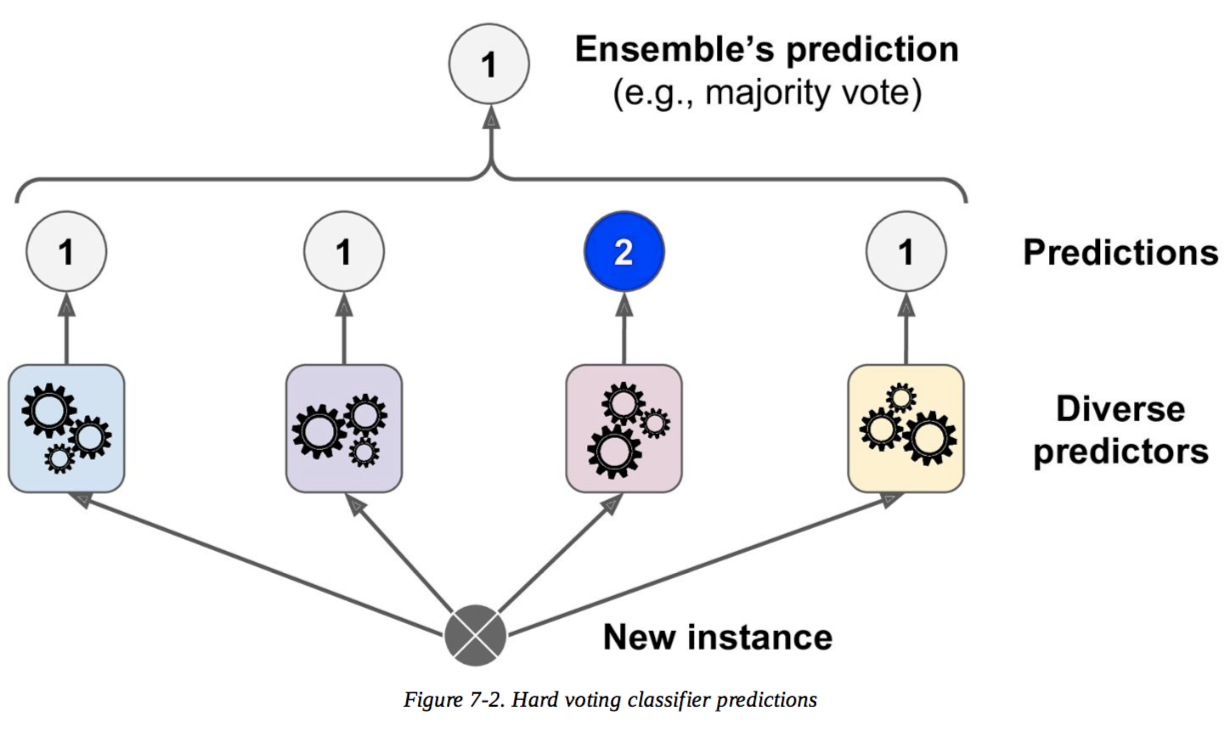Voting Classifier From “Hands on Machine Learning With Sci-kit Learn, Keras, and Tensorflow” (Géron).

We build three different base models: Gaussian naive Bayes, a random forest, and a support vector classifier. The naive Bayes and SVC models are wrapped in a pipeline with a StandardScaler, so scaling is re-fit on each training fold during cross-validation and never sees validation rows. The random forest works on raw features.

from sklearn.ensemble import RandomForestClassifier, VotingClassifier
from sklearn.metrics import accuracy_score
from sklearn.model_selection import cross_val_score
from sklearn.naive_bayes import GaussianNB
from sklearn.pipeline import make_pipeline
from sklearn.preprocessing import StandardScaler
from sklearn.svm import SVC

nb_clf = make_pipeline(StandardScaler(), GaussianNB())
rf_clf = RandomForestClassifier(random_state=42)
svc_clf = make_pipeline(StandardScaler(), SVC(random_state=42))

voting_clf = VotingClassifier(
    estimators=[('nb', nb_clf), ('rf', rf_clf), ('svc', svc_clf)],
    voting='hard')

Compare the ensemble with its members using 5-fold cross-validation — on the training set only.

for name, clf in [('Naive Bayes', nb_clf), ('Random Forest', rf_clf),
                  ('SVC', svc_clf), ('Voting ensemble', voting_clf)]:
    scores = cross_val_score(clf, X_train, y_train, scoring='accuracy', cv=5, n_jobs=-1)
    print(f"{name:16s} CV accuracy: {scores.mean():.3f} +/- {scores.std():.3f}")

Naive Bayes      CV accuracy: 0.784 +/- 0.010

Random Forest    CV accuracy: 0.877 +/- 0.014

SVC              CV accuracy: 0.880 +/- 0.012

Voting ensemble  CV accuracy: 0.875 +/- 0.011

Now fit the voting ensemble on the full training set and report its test accuracy — once.

voting_clf.fit(X_train, y_train)
voting_test = accuracy_score(y_test, voting_clf.predict(X_test))
print(f"Voting classifier test accuracy: {voting_test:.3f}")

Voting classifier test accuracy: 0.875

Note that taking the average of the predicted probability, instead of its max, is also a possibility. One can only evaluate the classifiers that output probabilities, which SVM does not do by default. Set voting to soft to compare with the mean probability.

2. Bagging and Pasting¶

This approach uses the same model algorithm but resamples the training set. For resampling with replacement (bootstrap), it is called bagging; for resampling without replacement, it is called pasting.

Several models are trained on different data, then the predictions are aggregated (statistical mode for classification and average for regression). The aggregated model tends to have lower variance than the individual models, similar to what a single model would get if it were trained on more data.

Below we bag 50 k-nearest-neighbor classifiers, each trained on a random half of the training rows. The bagger sits inside a scaler pipeline because kNN is scale-sensitive. Change n_estimators, max_samples, or bootstrap and watch the cross-validated score.

from sklearn.ensemble import BaggingClassifier
from sklearn.neighbors import KNeighborsClassifier

bag_clf = make_pipeline(
    StandardScaler(),
    BaggingClassifier(
        estimator=KNeighborsClassifier(),
        n_estimators=50,     # number of models to train
        max_samples=0.5,     # each model sees half of the training rows
        bootstrap=True,      # True: bagging; False: pasting
        n_jobs=-1,           # use all available CPU cores
    ))
scores = cross_val_score(bag_clf, X_train, y_train, cv=5)
print(f"Bagged kNN CV accuracy: {scores.mean():.3f}")

Bagged kNN CV accuracy: 0.841

Out-of-bag evaluation¶

Sampling with replacement has a useful side effect. When you draw $m$ samples with replacement from $m$ training rows, each bootstrap contains only about 63% of the unique rows; the other ~37% never enter that model’s training set. Those left-out rows form a free validation set for that model. Set oob_score=True and the BaggingClassifier scores each training row using only the models that never saw it.

from sklearn.tree import DecisionTreeClassifier

oob_clf = BaggingClassifier(
    estimator=DecisionTreeClassifier(),
    n_estimators=200,
    oob_score=True,
    random_state=42,
)
oob_clf.fit(X_train, y_train)
oob_test = accuracy_score(y_test, oob_clf.predict(X_test))
print(f"Out-of-bag score: {oob_clf.oob_score_:.3f}")
print(f"Test accuracy:    {oob_test:.3f}")

Out-of-bag score: 0.876
Test accuracy:    0.887

The two numbers are close, and they should be: the out-of-bag score is an honest estimate because every prediction comes from models that never trained on that row — the same property a held-out test set has.

Ensemble spread as uncertainty¶

The 200 bagged trees give more than a class label. Each tree casts a vote, and the split of the votes is itself a measurement: when 195 of 200 trees agree, the ensemble is confident; when the votes scatter across three classes, the ensemble is telling you it does not know. The fitted bagger keeps its trees in estimators_, so we can count the votes ourselves and attach a confidence to every test prediction, with no retraining.

import matplotlib.pyplot as plt

# per-tree predictions on the test set: one row per tree
tree_votes = np.stack([tree.predict(X_test.to_numpy())
                       for tree in oob_clf.estimators_])

# each tree predicts a class index; count the votes for each class
n_classes = len(oob_clf.classes_)
vote_frac = np.stack([(tree_votes == k).mean(axis=0)
                      for k in range(n_classes)], axis=1)
agreement = vote_frac.max(axis=1)  # fraction voting the winning class
errors = oob_clf.predict(X_test) != y_test.to_numpy()

edges = [0.25, 0.5, 0.7, 0.9, 1.001]
bin_labels = ['25-50%', '50-70%', '70-90%', '90-100%']
bin_idx = np.digitize(agreement, edges) - 1
error_rate = [errors[bin_idx == b].mean() for b in range(4)]
counts = [int((bin_idx == b).sum()) for b in range(4)]

fig, ax = plt.subplots(figsize=(6, 4))
ax.bar(bin_labels, error_rate)
for i, (e, n) in enumerate(zip(error_rate, counts)):
    ax.text(i, e + 0.005, f"n={n}", ha='center')
ax.set_xlabel('Vote agreement (fraction of trees voting the winning class)')
ax.set_ylabel('Misclassification rate on the test set')
ax.grid(alpha=0.3, axis='y')
plt.show()

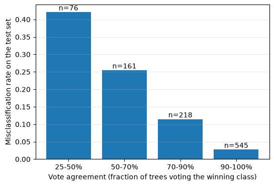
Trees that agree are usually right: above 90% agreement the ensemble is wrong about 3% of the time, while the samples that split the forest below 50% agreement are wrong about 40% of the time. The ensemble ranks its own predictions by trustworthiness before any label is revealed; in an operational catalog, the low-agreement events are the ones to route to an analyst.

The same recipe — train many models, read their disagreement as uncertainty — returns in lesson 4.5 as deep ensembles of neural networks.

3. Boosting¶

The idea behind boosting methods is to train predictors sequentially, each trying to correct its predecessor.

3.1 AdaBoost¶

The AdaBoost algorithm trains a new predictor by paying more attention to (up-weighting) the bad predictions from the previous predictor. For instance, in a classification, a first predictor will be underfitting the data and misclassifying labels. The second predictor weights more strongly the data that was misclassified. The learning_rate parameter sets the magnitude of that re-weighting.

AdaBoost works on any classifier that outputs class probabilities (e.g., decision trees, kNN; look for classifiers with a predict_proba() method). Here the weak learners are shallow trees (depth 2), which is the standard choice.

from sklearn.ensemble import AdaBoostClassifier

ada_clf = AdaBoostClassifier(
    estimator=DecisionTreeClassifier(max_depth=2),
    n_estimators=200,
    learning_rate=0.5,
    random_state=42,
)
ada_clf.fit(X_train, y_train)
ada_test = accuracy_score(y_test, ada_clf.predict(X_test))
print(f"AdaBoost test accuracy: {ada_test:.3f}")

AdaBoost test accuracy: 0.874

3.2 Gradient Boosting¶

Gradient boosting also builds trees sequentially, but each new tree fits the residuals of the current ensemble:

A single small tree is trained on the data (a weak learner).
A second small tree is trained on the residuals between the data and the first tree’s predictions. The residuals get smaller.
A third small tree fits the remaining residuals, and so on.
The final prediction is the sum of all the trees’ predictions.

n_estimators limits the total number of trees; too many trees overfit. The learning_rate scales the contribution of each tree; a lower rate needs more trees.

Gradient boosting won tabular machine learning. Histogram-based implementations — LightGBM, XGBoost, and scikit-learn’s HistGradientBoostingClassifier — bin the features to grow trees fast, and in 2026 they are the default choice for feature tables like this one. Random forests remain a strong, robust, nearly tuning-free baseline. Trees split on feature thresholds, so none of these models need scaled inputs.

First, scikit-learn’s built-in histogram gradient booster:

from sklearn.ensemble import HistGradientBoostingClassifier

hgb_clf = HistGradientBoostingClassifier(random_state=42)
hgb_clf.fit(X_train, y_train)
hgb_test = accuracy_score(y_test, hgb_clf.predict(X_test))
print(f"HistGradientBoosting test accuracy: {hgb_test:.3f}")

HistGradientBoosting test accuracy: 0.898

Then LightGBM, a widely used stand-alone library with the same scikit-learn interface:

from lightgbm import LGBMClassifier

lgbm_clf = LGBMClassifier(random_state=42, verbose=-1)
lgbm_clf.fit(X_train, y_train)
lgbm_test = accuracy_score(y_test, lgbm_clf.predict(X_test))
print(f"LightGBM test accuracy: {lgbm_test:.3f}")

LightGBM test accuracy: 0.892

4. Stacking¶

Voting treats every base model equally. Stacking instead trains a meta-learner on the base models’ predictions: it learns which model to trust, and where. The base models produce predictions; the meta-learner (often a simple logistic regression) takes those predictions as input features and fits them to the true labels.

There is a leakage trap here: if the meta-learner were trained on base-model predictions for rows the base models had already seen, it would learn to trust overfit predictions. scikit-learn’s StackingClassifier avoids this by generating the base predictions with internal cross-validation, so the meta-learner only ever sees each base model’s predictions on rows that model did not train on.

We stack three diverse bases — a random forest, a histogram gradient booster, and a scaled kNN — with a logistic regression on top.

from sklearn.ensemble import StackingClassifier
from sklearn.linear_model import LogisticRegression

base_estimators = [
    ('rf', RandomForestClassifier(random_state=42)),
    ('hgb', HistGradientBoostingClassifier(random_state=42)),
    ('knn', make_pipeline(StandardScaler(), KNeighborsClassifier())),
]

stack_clf = StackingClassifier(
    estimators=base_estimators,
    final_estimator=LogisticRegression(max_iter=1000),
    cv=5,
    n_jobs=-1,
)
stack_clf.fit(X_train, y_train)
stack_test = accuracy_score(y_test, stack_clf.predict(X_test))
print(f"Stacking test accuracy: {stack_test:.3f}")

Stacking test accuracy: 0.901

For comparison, a hard-voting ensemble of the same three bases on the same split:

voting3_clf = VotingClassifier(estimators=base_estimators, voting='hard', n_jobs=-1)
voting3_clf.fit(X_train, y_train)
voting3_test = accuracy_score(y_test, voting3_clf.predict(X_test))
print(f"Voting (same bases) test accuracy: {voting3_test:.3f}")

Voting (same bases) test accuracy: 0.891

Summary¶

Test accuracy and per-class recall for every ensemble in this lesson, against the trivial baseline. Aggregate accuracy hides class-specific failures; the recall columns show, for each true class, the fraction of its events the model catches.

from sklearn.metrics import recall_score

fitted = {
    'Voting (NB + RF + SVC)': voting_clf,
    'Bagged trees (OOB demo)': oob_clf,
    'AdaBoost': ada_clf,
    'HistGradientBoosting': hgb_clf,
    'LightGBM': lgbm_clf,
    'Stacking (RF + HGB + kNN)': stack_clf,
    'Voting (RF + HGB + kNN)': voting3_clf,
}
classes = sorted(y.unique())
rows = {'Majority-class baseline': [baseline] + [np.nan] * len(classes)}
for name, clf in fitted.items():
    pred = clf.predict(X_test)
    rows[name] = ([accuracy_score(y_test, pred)]
                  + list(recall_score(y_test, pred,
                                      average=None, labels=classes)))
results = pd.DataFrame(
    rows, index=['test accuracy'] + [f'recall: {c}' for c in classes]).T
results.round(3)

All ensembles clear the 25% floor by a wide margin, and the differences between the strong ensembles are small on this dataset. The recall columns show where the remaining errors live: every model catches noise and surface events at 90% recall or better, while explosion recall sits between 0.77 and 0.84 for all of them — aggregate accuracy hides a class that is misclassified two to three times as often as the others. The habit to keep: compare models by cross-validation inside the training set, spend the test set exactly once, and report per-class recall next to the aggregate score.

References¶

Kharita, A. (2024). Physical features for small sample of data (1000 events per class). Zenodo. 10.5281/ZENODO.14025693