3.2 Classification and Regression - Machine Learning in the Geosciences

Problems that need a quantitative response (numeric value) are regression; problems that need a qualitative response (boolean or category) are classification. Many statistical methods can be applied to both types of problems.

Binary classification has two output classes. They usually end up being “A” and “not A”. Examples are “earthquake” or “no earthquake=noise”. Multiclass classification refers to one with more than two classes.

Classification here requires that we know the labels, it is a form of supervised learning.

1. Classification Algorithms¶

There are several classifier algorithms, which we summarize below before practicing. For each one, ask three questions in this order: what geoscience question does it answer, what is the statistical idea behind it, and when does it suit your data? The scikit-learn names matter least — a coding agent can supply those.

Logistic Regression: Is this water sample potable? Is this waveform an earthquake or noise? Logistic regression draws a straight boundary through feature space and converts a sample’s distance from that boundary into a probability between 0 and 1. Because it outputs a probability rather than only a label, it suits problems where the answer must feed a forecast, and its coefficients can be read as the effect of each feature. Lesson 3.6 is devoted to it.
Linear Discriminant Analysis (LDA): Given density and magnetic susceptibility, is a rock specimen granite or basalt? LDA treats each class as a cloud of data samples with its own center but a shared spread, and finds the direction in feature space along which the class centers separate most cleanly relative to the scatter within each class; the decision boundary is a straight line between the projected clouds. Where PCA (Chapter 2.12) seeks the direction of largest variance regardless of class, LDA seeks the direction that best tells the classes apart. Because it estimates only class means and one common spread, it behaves well with small labeled collections — a few dozen specimens per rock type — where flexible models overfit.
Naive Bayes (NB): Which of three rock types most plausibly produced these measured properties? Naive Bayes asks, for each class, how probable the observed feature values would be if the sample belonged to that class — treating each feature as if it were independent of the others — and assigns the class that makes the observation most probable. That independence assumption is rarely true of geophysical measurements (temperature and humidity move together), yet the method often classifies well anyway, learns from very few data samples, and has almost nothing to tune.
K-nearest neighbors (KNN): If the training samples most similar to this one are mostly basalt, call it basalt. KNN stores the training data and classifies a new sample by a vote among its K closest neighbors in feature space. “Closest” depends on units — a density in kg/m³ would swamp a susceptibility measured in tiny SI values — so features in mixed units must be rescaled to comparable ranges first. The method assumes nothing about the shape of the class boundary, but it weakens as the number of features grows, and every prediction requires a search through the stored training set.
Support Vector Machine (SVM): Is this seismogram a quarry blast or a tectonic earthquake, when only a few hundred hand-labeled examples exist? SVM finds the boundary that separates the classes with the widest cushion — the margin — so that a data sample near the boundary would need a large perturbation to change side. Kernels (radial basis function, polynomial) let that boundary curve. SVM was the method of choice when labeled geoscience catalogs held hundreds of events rather than millions, and it remains strong in that small-sample regime; it returns a decision, not a probability.
Random Forest (RF): Does this combination of slope, rainfall, and lithology mark a hillslope as landslide-prone? A random forest grows many decision trees, each on a random subset of the data samples and features, and assigns the class that wins the vote across trees; averaging many noisy trees reduces the variance of any single one. It tolerates features in mixed units without rescaling and reports which features drove the classification, which is often the geoscientific question of interest. Its vote fractions look like probabilities but are not calibrated ones — lesson 3.6 returns to that.
Artificial Neural Networks (ANN): When the boundary between classes is too tangled for a line, a cushion, or a vote — telling eruption tremor from wind noise in a spectrogram — neural networks compose layers of simple functions into boundaries of nearly arbitrary shape. That flexibility is paid for in data: they need many more labeled samples than the methods above, and their decisions are harder to interpret. Chapter 4 treats them in depth.

Some classifiers can handle multiclass natively (Stochastic Gradient Descent - SGD; Random Forest classification; Naive Bayes). Others are strictly binary classifiers (Logistic Regression, Support Vector Machine classifier - SVM). In practice scikit-learn wraps binary classifiers in a one-vs-rest scheme automatically, so they still work on multiclass problems.

Exercise¶

We will create a synthetic dataset representing three rock types: Granite, Basalt, and Sandstone. Each type will have characteristic values for density and magnetic susceptibility.

🖥️ Lecture slides — Session 12 (Mon Oct 26)

import numpy as np
import pandas as pd
import matplotlib.pyplot as plt
from sklearn.dummy import DummyClassifier
from sklearn.model_selection import train_test_split
from sklearn.neighbors import KNeighborsClassifier
from sklearn.metrics import classification_report, confusion_matrix

Generate synthetic data


# Set random seed for reproducibility
np.random.seed(42)

# Number of samples per class
n_samples = 100

# Generate features for Granite
granite_density = np.random.normal(2.9, 0.2, n_samples)
granite_susceptibility = np.random.normal(0.0001, 0.0001, n_samples)
granite_label = ['Granite'] * n_samples

# Generate features for Basalt
basalt_density = np.random.normal(3.2, 0.2, n_samples)
basalt_susceptibility = np.random.normal(0.001, 0.0005, n_samples)
basalt_label = ['Basalt'] * n_samples

# Generate features for Sandstone
sandstone_density = np.random.normal(2.4, 0.2, n_samples)
sandstone_susceptibility = np.random.normal(0.00005, 0.00005, n_samples)
sandstone_label = ['Sandstone'] * n_samples

# Combine data
density = np.concatenate([granite_density, basalt_density, sandstone_density])
susceptibility = np.concatenate([granite_susceptibility, basalt_susceptibility, sandstone_susceptibility])
labels = np.concatenate([granite_label, basalt_label, sandstone_label])

# Create DataFrame
data = pd.DataFrame({
    'Density': density,
    'Magnetic Susceptibility': susceptibility,
    'Lithology': labels
})
data.head()

import seaborn as sns

sns.scatterplot(
    x='Density',
    y='Magnetic Susceptibility',
    hue='Lithology',
    data=data
)
plt.title('Rock Types Based on Density and Magnetic Susceptibility')
plt.show()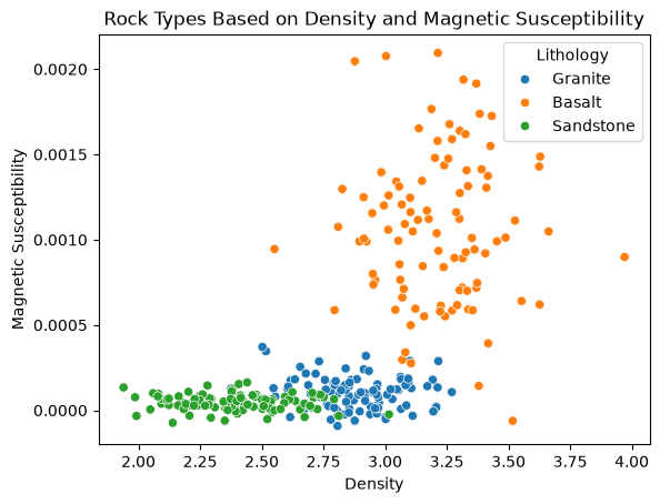

Split the data three ways: training, validation, and test (60/20/20). Each set has one job. The training set fits model parameters. The validation set compares models and tunes hyperparameters. The test set is touched once, at the very end, for the final honest estimate of performance.

X = data[['Density', 'Magnetic Susceptibility']]
y = data['Lithology']

# First split off the test set (20%), then split the rest into train (60%) and validation (20%)
X_temp, X_test, y_temp, y_test = train_test_split(
    X, y, test_size=0.2, random_state=42
)
X_train, X_val, y_train, y_val = train_test_split(
    X_temp, y_temp, test_size=0.25, random_state=42
)
print(f"train: {len(X_train)}, validation: {len(X_val)}, test: {len(X_test)}")

train: 180, validation: 60, test: 60

baseline = DummyClassifier(strategy="most_frequent")
baseline.fit(X_train, y_train)
print(f"Majority-class baseline accuracy on validation set: {baseline.score(X_val, y_val):.3f}")

Majority-class baseline accuracy on validation set: 0.333

Train a k-NN classifier on the training data. The number of neighbors $k$ is a hyperparameter: we try several values, score each on the validation set, and keep the best.

best_k, best_acc = None, 0.0
for k in [1, 3, 5, 9, 15]:
    clf = KNeighborsClassifier(n_neighbors=k)
    clf.fit(X_train, y_train)
    acc = clf.score(X_val, y_val)
    print(f"k = {k:2d}   validation accuracy = {acc:.3f}")
    if acc > best_acc:
        best_k, best_acc = k, acc
print(f"\nBest k on the validation set: {best_k}")

k =  1   validation accuracy = 0.683
k =  3   validation accuracy = 0.667
k =  5   validation accuracy = 0.700
k =  9   validation accuracy = 0.767
k = 15   validation accuracy = 0.750

Best k on the validation set: 9

Evaluate performance on the test set, once, with the chosen $k$ .

classifier = KNeighborsClassifier(n_neighbors=best_k)
classifier.fit(X_train, y_train)

y_pred = classifier.predict(X_test)
print(confusion_matrix(y_test, y_pred))
print(classification_report(y_test, y_pred))

[[12  4  0]
 [ 4 18  0]
 [ 1  3 18]]
              precision    recall  f1-score   support

      Basalt       0.71      0.75      0.73        16
     Granite       0.72      0.82      0.77        22
   Sandstone       1.00      0.82      0.90        22

    accuracy                           0.80        60
   macro avg       0.81      0.80      0.80        60
weighted avg       0.82      0.80      0.80        60

2. Regression Algorithms¶

Regression models predict continuous numerical values from inputs.

Example applications in the geosciences include predicting groundwater levels from climate and pumping records, estimating soil properties from spectral measurements, and statistical downscaling of temperature and precipitation.

2.1 Linear Regression¶

Let $y$ be the data, and $\hat{y}$ be the predicted value of the data. A general linear regression can be formulated as

$\hat{y} = w_0 + w_1 x_1 + ... + w_n x_n = h_w (\mathbf{x})$ .

$\mathbf{\hat{y}} = \mathbf{G} \mathbf{w}$ .

$y$ is a data vector of length $m$ , $\mathbf{x}$ is a feature vector of length $n$ . $\mathbf{w}$ is a vector of model parameter, $h_w$ is referred to as the hypothesis function or the model using the model parameter $w$ . In the most simple case of a linear regression with time, the formulation becomes:

$\hat{y} = w_0 + w_1 t$ ,

where $x_1 = t$ the time feature.

To evaluate how well the model performs, we will compute a loss score, or a residual. It is the result of applying a loss or cost or objective function to the prediction and the data. The most basic cost function is the Mean Square Error (MSE):

$MSE(\mathbf{x},h_w) = \frac{1}{m} \sum_{i=1}^{m} \left( h_w(\mathbf{x})_i - y_i \right)^2 = \frac{1}{m} \sum_{i=1}^{m} \left( \hat{y}_i - y_i \right)^2$ , in the case of a linear regression.

The Normal Equation is the solution to the linear regression that minimize the MSE.

$\mathbf{w} = \left( \mathbf{x}^T\mathbf{x} \right)^{-1} \mathbf{x}^T \mathbf{y}$

This compares with the classic inverse problem framed by $\mathbf{d} = \mathbf{G} \mathbf{m}$ .

$\mathbf{m} = \left( \mathbf{G}^T\mathbf{G} \right)^{-1} \mathbf{G}^T \mathbf{d}$

It can be solved using Numpy linear algebra module. If $\left( \mathbf{x}^T\mathbf{x} \right)$ is singular and cannot be inverted, a lower rank matrix called the pseudoinverse can be calculated using singular value decomposition. We also used in a previous class the Scikit-learn function for sklearn.linear_model.LinearRegression, which is the implementation of the pseudoinverse. We practice below how to use these standard inversions:

Other common algorithms¶

Beyond ordinary linear regression, common regression algorithms include:

Polynomial Regression: How fast does soil dry as temperature climbs, when the response bends rather than following a straight line? Adding squared and cross terms of the features lets the same least-squares machinery fit a curve. Low degrees are usually enough; high degrees oscillate wildly outside the range of the training samples, which is dangerous when the model will be asked about conditions it has never seen.
Support Vector Regression (SVR): The regression form of SVM. It fits a function while ignoring residuals smaller than a chosen tolerance, so only the data samples falling outside that band shape the fit. This makes it forgiving of measurement noise and less swayed by a single spiking sensor.
Random Forest Regression: How much rain fell, given these radar features? An ensemble of decision trees whose predictions are averaged; it captures curved relationships and interactions among features, with no rescaling needed for mixed units. One caution: a forest cannot predict beyond the range of its training targets, so it will never forecast a rainfall larger than any it was trained on.
Gradient-Boosted Trees: Trees added sequentially, each one fitting the residuals the previous ones left behind. On tabular geoscience data — station measurements, borehole logs, catalog attributes — boosted trees are often the most accurate choice, at the price of more hyperparameters to tune and a greater appetite for overfitting than a random forest.
Neural Networks: Fit relationships of nearly arbitrary shape, given enough data samples. For the small structured datasets of this chapter, the simpler methods above usually match them; Chapter 4 covers when they pull ahead.

Exercise¶

Objective: Predict soil moisture content based on environmental factors.

We will simulate soil moisture influenced by temperature and humidity.

# Seeded random generator for reproducibility
rng = np.random.default_rng(42)

# Number of samples
n_samples = 300

# Generate environmental variables
temperature = rng.uniform(15, 35, n_samples)  # in degrees Celsius
humidity = rng.uniform(30, 90, n_samples)     # in percentage

# Generate soil moisture as a function of temperature and humidity,
# with a mild quadratic term in temperature
soil_moisture = (
    0.5 * humidity
    - 0.3 * temperature
    - 0.02 * (temperature - 25) ** 2
    + rng.normal(0, 2, n_samples)
)

# Create DataFrame
data = pd.DataFrame({
    'Temperature': temperature,
    'Humidity': humidity,
    'Soil Moisture': soil_moisture
})
data.head()

The true function now has a mild nonlinearity (the quadratic term in temperature). This matters for the exercise: model selection is only meaningful when the true function is unknown. If the data were exactly linear, linear regression would win by construction and comparing models would teach nothing.

Data visualization


fig = plt.figure(figsize=(10, 7))
ax = fig.add_subplot(111, projection='3d')
ax.scatter(data['Temperature'], data['Humidity'], data['Soil Moisture'])
ax.set_xlabel('Temperature (°C)')
ax.set_ylabel('Humidity (%)')
ax.set_zlabel('Soil Moisture')
plt.tight_layout()
plt.show()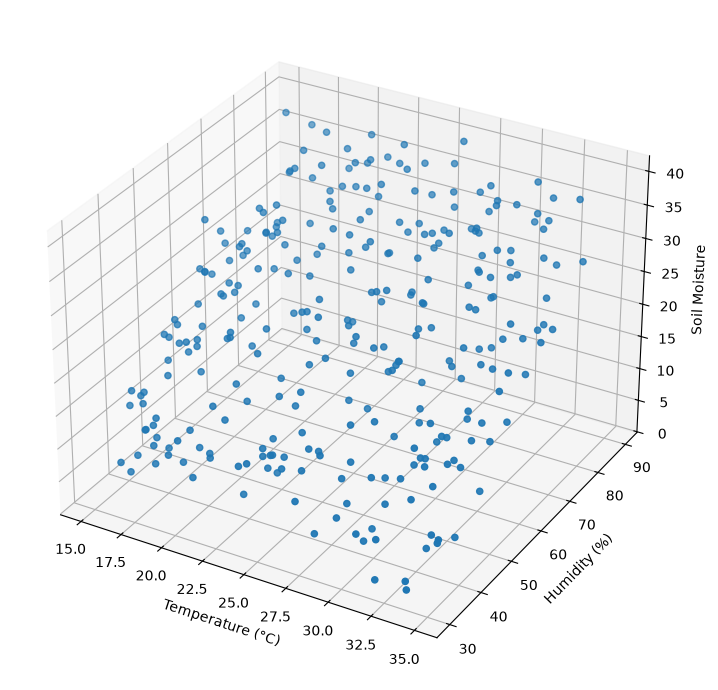

Split the data into training, validation, and test sets (60/20/20), same roles as before.

X = data[['Temperature', 'Humidity']]
y = data['Soil Moisture']

X_temp, X_test, y_temp, y_test = train_test_split(
    X, y, test_size=0.2, random_state=42
)
X_train, X_val, y_train, y_val = train_test_split(
    X_temp, y_temp, test_size=0.25, random_state=42
)
print(f"train: {len(X_train)}, validation: {len(X_val)}, test: {len(X_test)}")

train: 180, validation: 60, test: 60

Start with the trivial baseline: predict the mean of the training targets for every sample. Any regression model must beat it.

from sklearn.dummy import DummyRegressor
from sklearn.metrics import mean_squared_error, r2_score

baseline = DummyRegressor(strategy="mean")
baseline.fit(X_train, y_train)
y_val_base = baseline.predict(X_val)
print(f"Baseline (mean prediction) on validation set: "
      f"MSE = {mean_squared_error(y_val, y_val_base):.2f}, "
      f"R2 = {r2_score(y_val, y_val_base):.3f}")

Baseline (mean prediction) on validation set: MSE = 87.15, R2 = -0.012

Now the simplest real model: linear regression.

from sklearn.linear_model import LinearRegression

linreg = LinearRegression()
linreg.fit(X_train, y_train)
y_val_lin = linreg.predict(X_val)
mse_lin = mean_squared_error(y_val, y_val_lin)
print(f"Linear regression on validation set: "
      f"MSE = {mse_lin:.2f}, R2 = {r2_score(y_val, y_val_lin):.3f}")

Linear regression on validation set: MSE = 5.09, R2 = 0.941

Next, a degree-2 polynomial model: a pipeline that expands the features into all degree-2 terms, then fits a linear regression on them.

from sklearn.pipeline import Pipeline
from sklearn.preprocessing import PolynomialFeatures

polyreg = Pipeline([
    ("poly", PolynomialFeatures(degree=2)),
    ("linreg", LinearRegression()),
])
polyreg.fit(X_train, y_train)
y_val_poly = polyreg.predict(X_val)
mse_poly = mean_squared_error(y_val, y_val_poly)
print(f"Degree-2 polynomial on validation set: "
      f"MSE = {mse_poly:.2f}, R2 = {r2_score(y_val, y_val_poly):.3f}")

Degree-2 polynomial on validation set: MSE = 4.80, R2 = 0.944

Pick the model with the lower validation MSE, then report its performance once on the test set.

if mse_poly < mse_lin:
    best_name, best_model = "degree-2 polynomial", polyreg
else:
    best_name, best_model = "linear regression", linreg

y_test_pred = best_model.predict(X_test)
print(f"Selected model: {best_name}")
print(f"Test set: MSE = {mean_squared_error(y_test, y_test_pred):.2f}, "
      f"R2 = {r2_score(y_test, y_test_pred):.3f}")

Selected model: degree-2 polynomial
Test set: MSE = 4.02, R2 = 0.947

The polynomial model wins on the validation set because the true function contains a quadratic term the linear model cannot represent; the test score, used only once, confirms that choice.