3.7 Random Forests - Machine Learning in the Geosciences

1. Decision Trees¶

A decision tree is a supervised learning algorithm used for both classification and regression tasks. It is a flowchart-like structure where:

Internal nodes represent tests on features (attributes),
Branches represent the outcomes of these tests, and
Leaf nodes represent the final output or decision (such as a class label or a predicted value).

Each node in the tree splits the data into subsets based on feature values that minimize a certain cost function, such as Gini impurity or entropy for classification, and mean squared error for regression.

2. How Decision Trees Work

Splitting: The algorithm begins at the root node by selecting a feature that best splits the dataset according to a chosen criterion. For classification, common metrics are Gini impurity or information gain.
Recursive Partitioning: This process is recursively applied to the resulting subsets, creating branches of the tree. Each decision aims to simplify the problem by reducing uncertainty about the outcome.
Stopping Criteria: The algorithm continues until it reaches a stopping condition, which could be a minimum node size or a maximum tree depth, to prevent overfitting.
Prediction: Once the tree is trained, it can classify new data points by traversing the tree from the root to a leaf, following the decisions at each node.

3. Why Are Decision Trees Relevant in Geoscientific Research?

Decision trees are particularly useful in geoscientific research for several reasons:

Interpretability: Decision trees provide a clear, visual representation of how decisions are made. In geosciences, where models must often be explainable to a wide range of stakeholders (e.g., policymakers, environmentalists), decision trees allow users to understand and trust the predictions.
Handling Complex, Nonlinear Relationships: Geoscientific data, such as environmental or climate data, often exhibit complex relationships between variables. Decision trees can naturally capture these nonlinear relationships without the need for heavy data preprocessing.
Handling Missing Data: Decision trees can handle datasets with missing values, which is common in geoscience due to the challenges of continuous monitoring in harsh environments or remote locations.
Feature Importance: Decision trees rank the importance of each feature based on its contribution to the model. This is valuable in geosciences to identify which factors (e.g., temperature, precipitation, or seismic activity) have the most impact on a particular outcome (e.g., predicting landslides or earthquakes).
Scalability: Decision trees can be applied to large datasets, often found in geosciences, with minimal computational overhead. They can be adapted to distributed computing frameworks to handle vast geospatial datasets.

4. Geoscientific Applications

Seismic Event Classification: Decision trees can classify seismic events (e.g., earthquakes, volcanic eruptions) based on waveforms, frequency content, and other features.
Landslide Risk Prediction: They can model complex interactions between environmental variables like slope, soil type, and rainfall, identifying areas at higher risk of landslides.
Climate Classification and Prediction: Decision trees can be used to classify climate zones based on environmental variables or predict future climate patterns by analyzing historical weather data.

🖥️ Lecture slides — Session 17 (Fri Nov 6)

2. Random Forest¶

2.1 Concepts¶

1. What Are Random Forests?

A random forest is an ensemble learning method that builds on the foundation of decision trees. Instead of relying on a single decision tree, random forests combine the predictions of many decision trees to improve accuracy, robustness, and reduce overfitting. Each tree in the forest independently makes a prediction, and the forest aggregates these predictions—typically by majority voting for classification tasks or averaging for regression tasks—to make a final decision.

2. How Do Random Forests Work?

Bootstrap Aggregation (Bagging): Each decision tree in a random forest is trained on a different subset of the original dataset. This is achieved through bootstrapping, where random samples (with replacement) are drawn from the dataset for each tree. This diversity in training data allows trees to develop slightly different models, reducing the likelihood that all trees make the same errors.
Feature Randomness: At each split, a random subset of features is chosen for consideration, rather than the full feature set. This randomness decorrelates the trees from each other, further reducing the chance of overfitting and enhancing generalization.
Prediction Aggregation: Once all trees in the forest have made their predictions, random forests aggregate these to produce a final output. For classification, it’s usually a majority vote across trees; for regression, the final output is the average prediction across trees.

3. Why Random Forests Are Valuable in Geoscientific Research

Random forests address some limitations of single decision trees, making them particularly useful for geoscientific applications:

Increased Accuracy and Reduced Overfitting: The ensemble approach of random forests typically improves prediction accuracy over a single decision tree. This matters in geosciences, where data can be noisy, and precise predictions are required for applications like hazard assessment.
Better Generalization: Random forests generalize better than single trees due to the diversity in the ensemble. This means that random forests are more likely to perform well on new, unseen data, which is vital in dynamic geoscientific contexts (e.g., changing climate patterns or evolving geological conditions).
Feature Importance and Interpretability: Like decision trees, random forests provide feature importance scores, indicating which features contribute most to predictions. This helps geoscientists identify key drivers of a phenomenon, such as factors leading to landslides or influencing seismic activity.
Scalability: Random forests are highly scalable and can be distributed across multiple processors, making them suitable for large geospatial datasets commonly encountered in geoscience, such as remote sensing data.

2.2 Practice¶

We will train a random forest to predict today’s maximum temperature at a Seattle-like site from a few simple features: yesterday’s temperature, the temperature two days ago, the historical average for the calendar day, and the date itself.

Earlier editions of this book downloaded a temps.csv file from a Google Docs link. That link is dead, and the file carried a joke friend column (a random guess within 20 degrees of the average). The 2026 edition generates an equivalent daily record in-notebook, so we know its exact structure: a seasonal cycle, a weak warming trend, and autocorrelated weather noise. The same dataset returns in lesson 3.10, so results are directly comparable across the two lessons.

The workflow below follows the spirit of Will Koehrsen’s random forest tutorial, updated for current practice.

import numpy as np
import pandas as pd


def make_daily_temps(start="2012-01-01", end="2019-12-31", seed=42):
    """Synthetic Seattle-like daily maximum temperature record (degrees F).

    Seasonal climatology + a weak warming trend + AR(1) weather noise.
    Generated in-notebook so the lesson does not depend on a remote file.
    """
    rng = np.random.default_rng(seed)
    dates = pd.date_range(start, end, freq="D")
    day_of_year = dates.dayofyear.to_numpy()
    climatology = 62.0 - 15.0 * np.cos(2 * np.pi * (day_of_year - 203) / 365.25)
    trend = 0.05 * np.arange(len(dates)) / 365.25
    noise = np.zeros(len(dates))
    for i in range(1, len(dates)):
        noise[i] = 0.65 * noise[i - 1] + rng.normal(0.0, 3.0)
    df = pd.DataFrame(
        {
            "date": dates,
            "average": np.round(climatology, 1),  # historical average for that calendar day
            "actual": np.round(climatology + trend + noise, 1),
        }
    )
    df["temp_1"] = df["actual"].shift(1)  # yesterday's max
    df["temp_2"] = df["actual"].shift(2)  # two days ago
    df["month"] = df["date"].dt.month
    df["day"] = df["date"].dt.day
    df["doy_sin"] = np.sin(2 * np.pi * day_of_year / 365.25)
    df["doy_cos"] = np.cos(2 * np.pi * day_of_year / 365.25)
    return df.dropna().reset_index(drop=True)


df = make_daily_temps()
print(df.shape)
df.head()

(2920, 9)

# Descriptive statistics for each column
df.describe()

Exploring the data¶

Before any modeling, look at the series. We plot the target (actual), the strongest lag feature (temp_1), and the climatology (average). The seasonal cycle dominates; the weather noise rides on top of it.

import matplotlib.pyplot as plt

fig, axes = plt.subplots(nrows=3, ncols=1, figsize=(10, 8), sharex=True)

axes[0].plot(df["date"], df["actual"], lw=0.6, color="tab:blue")
axes[0].set_ylabel("Temperature (F)")
axes[0].set_title("Actual daily max temperature")

axes[1].plot(df["date"], df["temp_1"], lw=0.6, color="tab:orange")
axes[1].set_ylabel("Temperature (F)")
axes[1].set_title("Yesterday's max temperature (temp_1)")

axes[2].plot(df["date"], df["average"], lw=0.8, color="tab:green")
axes[2].set_ylabel("Temperature (F)")
axes[2].set_title("Historical average for the calendar day")
axes[2].set_xlabel("Date")

plt.tight_layout()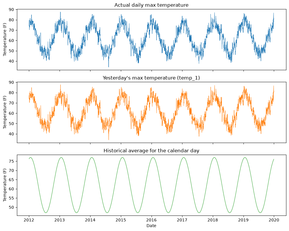

Splitting into training and test sets¶

The target is actual. The features are the two lags, the climatology, and the date encoded as month, day, and a sine/cosine pair for the day of year.

from sklearn.model_selection import train_test_split

features = ["temp_1", "temp_2", "average", "month", "day", "doy_sin", "doy_cos"]
X = df[features]
y = df["actual"]

X_train, X_test, y_train, y_test = train_test_split(X, y, test_size=0.25, random_state=42)
print("Training features:", X_train.shape)
print("Testing features: ", X_test.shape)

Training features: (2190, 7)
Testing features:  (730, 7)

The baseline: climatology¶

from sklearn.metrics import mean_absolute_error, root_mean_squared_error, r2_score

baseline_pred = X_test["average"]
baseline_mae = mean_absolute_error(y_test, baseline_pred)
baseline_rmse = root_mean_squared_error(y_test, baseline_pred)
print(f"Climatology baseline:  MAE = {baseline_mae:.2f} F,  RMSE = {baseline_rmse:.2f} F")

Climatology baseline:  MAE = 3.25 F,  RMSE = 4.10 F

Fitting a random forest¶

We fit a forest of 300 trees on the training set and score it on the held-out test set.

import time
from sklearn.ensemble import RandomForestRegressor

rf = RandomForestRegressor(n_estimators=300, random_state=42)

t0 = time.perf_counter()
rf.fit(X_train, y_train)
rf_fit_time = time.perf_counter() - t0

rf_pred = rf.predict(X_test)
rf_mae = mean_absolute_error(y_test, rf_pred)
rf_rmse = root_mean_squared_error(y_test, rf_pred)
rf_r2 = r2_score(y_test, rf_pred)
print(f"Random forest (test): MAE = {rf_mae:.2f} F,  RMSE = {rf_rmse:.2f} F,  R2 = {rf_r2:.3f}")
print(f"Fit time: {rf_fit_time:.2f} s")

Random forest (test): MAE = 2.55 F,  RMSE = 3.21 F,  R2 = 0.923
Fit time: 1.94 s

Cross-validation instead of a single split¶

A single train/test split is one random draw; cross-validation shows the spread. We run 5-fold cross-validation on the training data only, keeping the test set untouched.

from sklearn.model_selection import KFold, cross_val_score

cv = KFold(n_splits=5, shuffle=True, random_state=42)
rf_cv_scores = -cross_val_score(
    RandomForestRegressor(n_estimators=300, random_state=42),
    X_train, y_train, cv=cv, scoring="neg_mean_absolute_error",
)
print(f"Random forest 5-fold CV MAE: {rf_cv_scores.mean():.2f} +/- {rf_cv_scores.std():.2f} F")

Random forest 5-fold CV MAE: 2.59 +/- 0.03 F

Feature importances¶

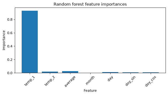
Random forests rank features by how much they reduce the splitting criterion across all trees. This is a quick, model-internal view of which inputs matter — computed on the training data, with biases we examine below.

importances = rf.feature_importances_

# Print features sorted by importance
for name, imp in sorted(zip(features, importances), key=lambda pair: pair[1], reverse=True):
    print(f"{name:10s} importance: {imp:.3f}")

fig, ax = plt.subplots(figsize=(7, 4))
ax.bar(features, importances)
ax.set_ylabel("Importance")
ax.set_xlabel("Feature")
ax.set_title("Random forest feature importances")
plt.xticks(rotation=45)
plt.tight_layout()

temp_1     importance: 0.929
average    importance: 0.025
temp_2     importance: 0.018
day        importance: 0.010
doy_cos    importance: 0.009
doy_sin    importance: 0.007
month      importance: 0.001

# Retrain using only the two most important features, chosen programmatically
top2 = [features[i] for i in np.argsort(importances)[::-1][:2]]
print("Top-2 features:", top2)

rf_top2 = RandomForestRegressor(n_estimators=300, random_state=42)
rf_top2.fit(X_train[top2], y_train)
top2_pred = rf_top2.predict(X_test[top2])
top2_mae = mean_absolute_error(y_test, top2_pred)

print(f"Full model (7 features)  test MAE: {rf_mae:.2f} F")
print(f"Top-2 model              test MAE: {top2_mae:.2f} F")

Top-2 features: ['temp_1', 'average']

Full model (7 features)  test MAE: 2.55 F
Top-2 model              test MAE: 2.69 F

Two features recover most of the skill of seven: when a compact model performs nearly as well, prefer it — it is cheaper to run, easier to explain, and less likely to overfit.

Interpreting importances¶

The impurity importances above are a property of the fitted trees, not of the world. They are computed on the training data, and when features are correlated the trees split the credit among them depending on which one a node happened to pick. Permutation importance asks a different question: how much does the held-out score degrade when one feature’s values are shuffled? Computed on the test set, it measures what the model actually relies on for new data.

from sklearn.inspection import permutation_importance

perm = permutation_importance(
    rf, X_test, y_test, n_repeats=20, random_state=42,
    scoring="neg_mean_absolute_error",
)

fig, (ax1, ax2) = plt.subplots(1, 2, figsize=(11, 4))
order = np.argsort(importances)
ax1.barh(np.array(features)[order], importances[order])
ax1.set_title("Impurity importance (training)")
order = np.argsort(perm.importances_mean)
ax2.barh(np.array(features)[order], perm.importances_mean[order],
         xerr=perm.importances_std[order])
ax2.set_title("Permutation importance (test set)")
ax2.set_xlabel("Increase in test MAE (F) when shuffled")
plt.tight_layout()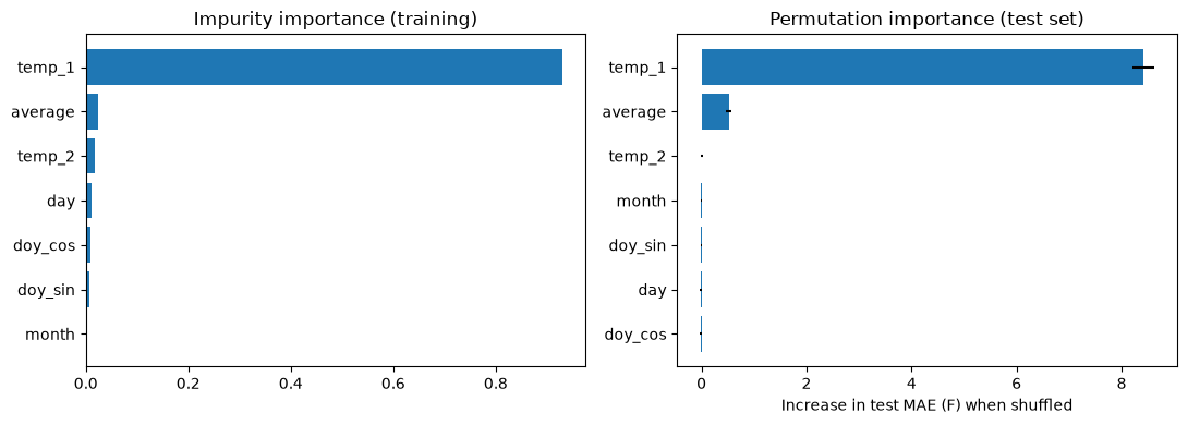

Here the two rankings agree that temp_1 and average dominate, but that agreement is not guaranteed. To see how correlated features mislead the impurity ranking, add one that carries no new information at all: temp_1 converted to Celsius, a perfect copy up to units.

X_train_dup = X_train.copy()
X_test_dup = X_test.copy()
X_train_dup["temp_1_C"] = (X_train_dup["temp_1"] - 32) * 5 / 9
X_test_dup["temp_1_C"] = (X_test_dup["temp_1"] - 32) * 5 / 9

rf_dup = RandomForestRegressor(n_estimators=300, random_state=42).fit(X_train_dup, y_train)
dup_mae = mean_absolute_error(y_test, rf_dup.predict(X_test_dup))
print(f"Test MAE without the duplicate: {rf_mae:.2f} F,  with: {dup_mae:.2f} F")

comparison = pd.DataFrame({
    "without duplicate": pd.Series(importances, index=features),
    "with duplicate": pd.Series(rf_dup.feature_importances_, index=X_train_dup.columns),
}).round(3)
print(comparison)

Test MAE without the duplicate: 2.55 F,  with: 2.55 F
          without duplicate  with duplicate
average               0.025           0.025
day                   0.010           0.010
doy_cos               0.009           0.009
doy_sin               0.007           0.007
month                 0.001           0.001
temp_1                0.929           0.495
temp_1_C                NaN           0.435
temp_2                0.018           0.018

The predictions barely move, but temp_1’s importance is now split with its Celsius twin: at each node the trees pick whichever copy is offered. Nothing about yesterday’s temperature became less informative — only the bookkeeping changed. The notebook’s own features already correlate this way (temp_1 with temp_2 through day-to-day persistence, average with the doy_sin/doy_cos pair), so read any importance ranking as how this model distributes credit among the inputs it was given, not as a measurement of the world.

Partial dependence¶

A partial dependence plot shows how the model’s prediction changes as one feature varies, averaging over the others. We plot it for the top feature.

from sklearn.inspection import PartialDependenceDisplay

disp = PartialDependenceDisplay.from_estimator(rf, X_test, ["temp_1"])
disp.axes_[0, 0].set_ylabel("Predicted max temperature (F)")
plt.gcf().set_size_inches(5, 4)
plt.tight_layout()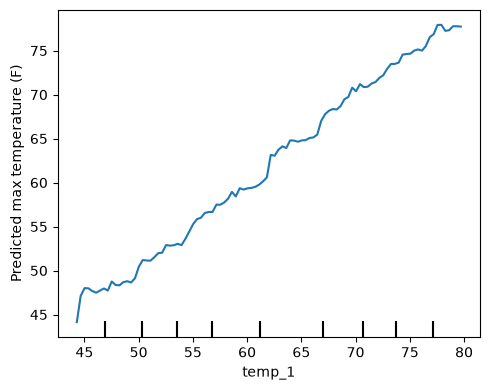

The prediction rises nearly linearly with yesterday’s temperature, which matches the AR(1) persistence built into the data. One caveat applies to everything in this section: importance is not causation — it reports what the model uses to predict, not what drives the temperature; shuffling temp_1 breaks the model, not the weather.

Comparison: gradient boosting¶

HistGradientBoostingRegressor builds trees sequentially, each one correcting the residuals of the last. We evaluate it with the same split and the same 5-fold cross-validation.

from sklearn.ensemble import HistGradientBoostingRegressor

hgb = HistGradientBoostingRegressor(random_state=42)

t0 = time.perf_counter()
hgb.fit(X_train, y_train)
hgb_fit_time = time.perf_counter() - t0

hgb_pred = hgb.predict(X_test)
hgb_mae = mean_absolute_error(y_test, hgb_pred)
hgb_rmse = root_mean_squared_error(y_test, hgb_pred)
hgb_r2 = r2_score(y_test, hgb_pred)

hgb_cv_scores = -cross_val_score(
    HistGradientBoostingRegressor(random_state=42),
    X_train, y_train, cv=cv, scoring="neg_mean_absolute_error",
)

print(f"Gradient boosting (test): MAE = {hgb_mae:.2f} F,  RMSE = {hgb_rmse:.2f} F,  R2 = {hgb_r2:.3f}")
print(f"Gradient boosting 5-fold CV MAE: {hgb_cv_scores.mean():.2f} +/- {hgb_cv_scores.std():.2f} F")
print(f"Fit times: random forest {rf_fit_time:.2f} s,  gradient boosting {hgb_fit_time:.2f} s")

Gradient boosting (test): MAE = 2.53 F,  RMSE = 3.20 F,  R2 = 0.923
Gradient boosting 5-fold CV MAE: 2.58 +/- 0.04 F
Fit times: random forest 1.94 s,  gradient boosting 0.14 s

Gradient boosting is the 2026 default for tabular regression: on feature tables it usually matches or beats a random forest at equal or lower training cost, and its advantage grows with dataset size. On a table this small the timings are close and can go either way. The random forest remains a strong, robust baseline that needs almost no tuning, which is why we teach it first.

Predictions against observations¶

Finally, plot the test-set predictions on top of the full observed series.

test_dates = df.loc[X_test.index, "date"]

fig, ax = plt.subplots(figsize=(10, 4))
ax.plot(df["date"], df["actual"], "-", lw=0.5, color="tab:blue", label="actual")
ax.plot(test_dates, rf_pred, ".", ms=3, color="tab:red", label="RF prediction (test)")
ax.set_xlabel("Date")
ax.set_ylabel("Maximum temperature (F)")
ax.set_title("Test-set predictions and observed values")
ax.legend()
plt.tight_layout()

print(f"Climatology baseline MAE: {baseline_mae:.2f} F  |  Random forest MAE: {rf_mae:.2f} F")

Climatology baseline MAE: 3.25 F  |  Random forest MAE: 2.55 F

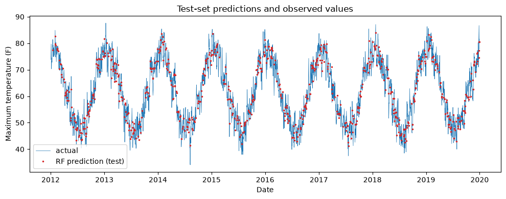
The forest beats the climatology baseline by a clear margin, so the lag features carry real information about tomorrow’s weather beyond the seasonal cycle. That comparison, not the score alone, is the evidence that the model learned something.