3.6 Logistic regression

Warning! Although it is called logistic regression, logistic regression is actually a classification method.

By Ariane Ducellier (2021)

🖥️ Lecture slides — Session 16 (Wed Nov 4)

In this lab, we are going to talk about:

• A simple classification method: Logistic regression
• Gradient descent method
• Automatic differentiation
• Introduction to PyTorch

Logistic regression¶

Remember linear regression:

$y = b + x w + \epsilon$

$y$ is a vector of length $n$, $x$ is a matrix with $n$ rows and $p$ columns, corresponding to $n$ observations and $p$ features that are used to explain $y$.

$b$ is a scalar. $w$ is a vector of length $p$. ε is a random error vector, of length $n$. It is independent of $x$, and has mean of zero.

Our objective is to find the best values of $b$ and $w$ so that the values of $\hat{y} = b + x w$ are as close as possible to the actual values $y$.

For linear regression, $y$ is a quantitative variable. What if $y$ is a qualitative variable, for example $y = 0$ for “no”, and $y = 1$ for “yes”?

One way to use regression to solve a classification problem is to model the probability of the variable $y$ taking the value 1:

$P (y = 1) = b + x w$

Once we have found the best values $\hat{b}$ and $\hat{w}$, we compute $\hat{y} = \hat{b} + x \hat{w}$. If $\hat{y} \geq 0.5$, we decide to classify this observation as $y = 1$, that is “yes”. If $\hat{y} < 0.5$, we decide to classify this observation as $y = 0$, that is “no”.

There is a problem with this method. We would like to have $0 \leq P (y = 1) \leq 1$ because it is a probability. However, there is nothing in this formulation that forces $b$ and $w$ to take values such that $\hat{y} = \hat{b} + x \hat{w}$ will always take values in $[0, 1]$.

To solve this problem, we can instead write:

$z = b + x w$ and $P (y = 1) = \frac{1}{1 + e^{-z}}$

That way, we always have $0 \leq P (y = 1) \leq 1$. When $b + x w$ gets large, $P (y = 1)$ gets close to 1, and the value “yes” is more and more likely. When $b + x w$ gets small, $P (y = 1)$ gets close to 0, and the value “no” is more and more likely.

How do we find the optimal value of $b$ and $w$? We define the cross-entropy loss function. For one observation, the loss function is:

$\mathcal{L} = - \left(y_i \log \hat{y}_i + (1 - y_i) \log (1 - \hat{y}_i)\right)$ with $\hat{y}_i = \frac{1}{1 + e^{- (b + x_i^T w)}}$ where $x_i$ is the $i$th row of x.

If the true observation $y_i$ is 1 (“yes”) and $\hat{y}_i = 1$, the loss function takes the value 0. If $\hat{y}_i = 0$, the loss function tends to infinity.

If the true observation $y$ is 0 (“no”) and $\hat{y}_i = 0$, the loss function takes the value 0. If $\hat{y}_i = 1$, the loss function tends to infinity.

For all the $n$ observations, we write:

$\mathcal{L} = \sum_{i = 1}^n \mathcal{L}_i$

Our objective is thus to find the values of $b$ and $w$ that minimize the loss function. Note that with this formulation, $\mathcal{L}$ is always positive.

Gradient descent¶

We know that the gradient $\frac{\partial \mathcal{L}}{\partial w_j}$ is positive if the loss $\mathcal{L}$ increases when $w_j$ increases. Reversely, the gradient $\frac{\partial \mathcal{L}}{\partial w_j}$ is negative if the loss $\mathcal{L}$ decreases when $w_j$ increases.

To obtain smaller and smaller values of the loss, at each iteration we take:

$w_j^{(k + 1)} = w_j^{(k)} - \alpha \frac{\partial \mathcal{L}}{\partial w_j}$ for $j = 1 , \cdots , p$

$b^{(k + 1)} = b^{(k)} - \alpha \frac{\partial \mathcal{L}}{\partial b}$

We assume that the value of α is not too big. If the gradient is positive, then the value of $w_j$ will decrease at each iteration, and the value of the loss function will decrease. If the gradient is negative, then the value of $w_j$ will increase at each iteration, and the value of the loss will decrease.

So now, all we need to do is to compute the gradient of the loss function.

Automatic differentiation¶

There are three ways of computing the gradient. The first method is to use the formula of the loss:

$\mathcal{L} (w_j , b) = - \sum_{i = 1}^n y_i \log (\frac{1}{1 + \exp (- b - \sum_{j = 1}^p w_j x_{i,j})}) + (1 - y_i) \log (1 - \frac{1}{1 + \exp (- b - \sum_{j = 1}^p w_j x_{i,j})})$

and to calculate the exact formula of the derivatives $\frac{\partial \mathcal{L}}{\partial w_j}$ and $\frac{\partial \mathcal{L}}{\partial b}$. You just then have to implement the exact formula in the code to compute the gradient.

When the formula gets more and more complicated, you become more and more likely to make a mistake, either in the calculation of the derivative formula, either in the implementation in your code.

The second method is to compute an approximation of the gradient:

$\frac{\partial \mathcal{L}}{\partial w_j} = \frac{\mathcal{L}(w_j + \Delta w_j) - \mathcal{L}(w_j)}{\Delta w_j}$

If you write too many approximations, the method may not work very well and give inexact results.

The third method is to use automatic differentiation. If we write:

$z = x_i^T w + b = f_x(w, b)$, $\sigma = \frac{1}{1 + e^{-z}} = g(z)$ and $L = - (y_i \log(\sigma) + (1 - y_i) \log(1 - \sigma)) = h_y(\sigma)$, we get:

$\frac{\partial L}{\partial w_j} = \frac{\partial f}{\partial w_j} g'(z) h'(\sigma)$

It is very easy to compute the exact formula of the derivatives:

$\frac{\partial f}{\partial w_j}(w, b) = x_{i,j}$

$g'(z) = \frac{e^{-z}}{(1 + e^{-z})^2}$

$h'(\sigma) = - \frac{y_i}{\sigma} + \frac{1 - y_i}{1 - \sigma}$

When computing $L$, we thus need to keep in memory the values of $\frac{\partial f}{\partial w_j}(w, b)$, $g'(z)$, and $h'(\sigma)$ to be able to compute the gradient. That is what PyTorch is doing.

Introduction to PyTorch¶

PyTorch (https://pytorch.org/) is a Python package which allows you to build and train neural networks. It is based on automatic differentiation.

The data: water potability¶

We use a table of water-quality measurements with a binary target, Potability (0 = not potable, 1 = potable). Each row has 9 numeric features (pH, hardness, dissolved solids, and so on).

Some rows have missing values. We drop them and reset the row index.

Split before you scale¶

We set aside 30% of the rows as a test set before doing anything else. We fit the scaler on the training rows only and apply it to both sets: if the scaler saw the test rows, information about the test set would leak into training, and the final evaluation would no longer be honest.

Before training anything, compute the trivial baseline: a “model” that always predicts the most common class. Any classifier worth keeping must beat this number.

One observation, by hand¶

We are going to compute the loss corresponding to the first observation in the training set. Instead of using Numpy arrays to put our data and parameters, we are going to use torch tensors, because they have properties that Numpy arrays do not have.

This is the features of the first training observation:

This is the class of the first training observation:

Let us take random values for $w$ and $b$. When creating these variables, we use the option requires_grad=True because we will later want to compute the gradient with respect to these variables.

Let us define $z = f(w, b) = x_i^T w + b$. We have $\frac{\partial f}{\partial w_j} = x_{i,j}$ and $\frac{\partial f}{\partial b} = 1$.

By default, PyTorch only keeps gradients for leaf tensors like W and B. Intermediate tensors such as $z$ do not keep their gradients; calling retain_grad() asks PyTorch to store them so we can inspect them after the backward pass.

Let us define $\sigma = g(z) = \frac{1}{1 + e^{-z}} = g(f(w, b)) = (g \circ f) (w, b)$. We have $g'(z) = \frac{e^{-z}}{(1 + e^{-z})^2}$.

Note that here we use the function torch.exp instead of numpy.exp. That is because numpy just calculate the value of $e^x$ but does not know that the derivative of $e^x$ is $e^x$. If we want to be able to use automatic differentiation, we need to use the equivalent torch function that will compute both $\sigma(z)$ and $\frac{\partial \sigma}{\partial z}(z)$. This last value will be necessary and we will later compute the gradient.

Let us define $L = h(\sigma) = - (y_i \log(\sigma) + (1 - y_i) \log(1 - \sigma)) = h(g(z)) = h(g(f(w, b))) = (h \circ g \circ f) (w, b)$. We have $L'(\sigma) = - (\frac{y_i}{\sigma} - \frac{1 - y_i}{1 - \sigma})$.

We can now compute the gradient of the loss for one observation. This command computes the gradient of L with respect to all the variables that keep a gradient, that is W, B, z, and sigma, but it does not return the value.

We have $\frac{\partial L}{\partial \sigma} = - (\frac{y_i}{\sigma} - \frac{1 - y_i}{1 - \sigma})$. Let us compare the result from PyTorch with the exact mathematical formula.

We have $\frac{\partial L}{\partial z} = g'(z) h'(g(z))$ that is $\frac{\partial L}{\partial z} = g'(z) h'(\sigma)$. Let us compare the result from PyTorch with the exact mathematical formula.

We have $\frac{\partial L}{\partial b} = \frac{\partial f}{\partial b} g'(f(w, b)) h'(g(f(w, b)))$ that is $\frac{\partial L}{\partial b} = \frac{\partial f}{\partial b} g'(z) h'(\sigma)$. Similarly, we have $\frac{\partial L}{\partial w_j} = \frac{\partial f}{\partial w_j} g'(f(w, b)) h'(g(f(w, b)))$ that is $\frac{\partial L}{\partial w_j} = \frac{\partial f}{\partial w_j} g'(z) h'(\sigma)$. Let us compare the results from PyTorch with the exact mathematical formulas.

Implementation of logistic regression¶

Let us now implement logistic regression using the whole training set.

We could code the update rule $w^{(k+1)} = w^{(k)} - \alpha \, \partial \mathcal{L} / \partial w$ by hand, and earlier editions of this book did, with retain_grad bookkeeping at every step. torch.optim.SGD does exactly that update rule, so we let it handle the parameter updates and keep the loss formula explicit. We write the binary cross-entropy out in full rather than calling torch.nn.BCELoss — the point here is transparency, not convenience.

Two practical details:

• We clamp σ away from 0 and 1 before taking logs, so the loss never returns log(0).
• We stop when the relative change in the loss drops below 10^-6, or after 2000 iterations.

Plot the loss curve. It should decrease quickly at first, then flatten.

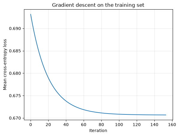
Evaluation on the test set¶

We now predict on both the training set and the test set. Earlier editions of this lesson evaluated the model on the same data it was trained on; the gap between the two numbers below is exactly why that overstates skill.

Let us now compute some classification metrics by hand, on the test set. N_test is the number of test observations.

Now compare training accuracy against test accuracy, next to the majority-class baseline.

Logistic regression barely beats the majority-class baseline on this table, and the recall on the potable class is low. That is an honest result: these 9 features, combined linearly, carry little signal about the target. A near-null result reported against a baseline is more useful than an inflated training-set score. If someone reports only a training accuracy, ask what the baseline was and what a held-out test set says.

Are the probabilities honest?¶

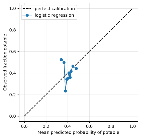
Everything above thresholds the sigmoid output at 0.5 and scores the resulting labels. But the model outputs a probability, and in many applications the probability itself is what you hand over. A classifier is calibrated when its stated probabilities match observed frequencies: among all test samples where the model says “70% chance potable”, about 70% should be potable.

Two tools measure this on the test set:

• A reliability diagram (sklearn.calibration.calibration_curve) bins the samples by predicted probability and plots the observed fraction of positives in each bin against the mean predicted probability. A calibrated model tracks the diagonal.
• The Brier score is the mean squared error of the probability, $\frac{1}{N} \sum_{i=1}^N (\hat{y}_i - y_i)^2$. Lower is better. Unlike accuracy, which only sees which side of 0.5 a prediction falls on, the Brier score punishes a wrong 0.99 much harder than a wrong 0.55.

The model’s probabilities span only about 0.27 to 0.57: it never claims certainty about any sample, which is consistent with the weak signal in these features. The curve wobbles around the diagonal, with most of the middle bins sitting below it — where the model says 40% potable, the observed frequency is closer to 30–40%, a mild overconfidence toward the potable class. Each quantile bin holds about 60 test samples, so each observed fraction carries sampling noise of roughly ±0.06, and only departures larger than that deserve interpretation. Verdict: roughly honest, weakly informative. The probabilities are usable, but they mostly restate the base rate.

A confident competitor, and how to repair it¶

A predict_proba method is no guarantee that the numbers coming out of it deserve to be called probabilities. Take a small random forest: 10 deep trees, each of which nearly memorizes the training set. Its “probability” of potable is the fraction of trees voting potable, and with 10 overfit trees those fractions easily land on extreme values like 0.9 or 1.0.

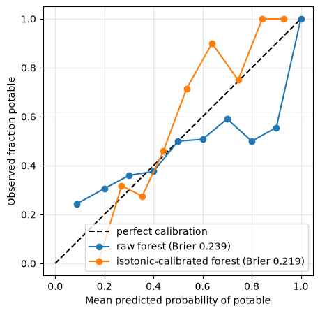
The forest memorizes the training set and still beats the logistic model on test accuracy. Now check whether its probabilities can be trusted, and repair them if not. The stakes are practical: when a model tells a hazard office “80% chance”, about 80% of those cases should come true, or the number is not a forecast anyone can act on. The repair re-labels the model’s scores using observed frequencies: hold some data samples out, record how often the samples scored near 0.9 actually turn out potable, and correct each score to that observed frequency. Only order-preserving corrections are allowed — if the forest scored sample A above sample B, the corrected probability of A stays at or above that of B — so the ranking of the samples survives; only the numbers attached to it change. CalibratedClassifierCV supplies the held-out samples by refitting the forest on cross-validation folds (the rotating splits of lesson 3.8), and scikit-learn’s name for the order-preserving fit is isotonic regression (method='isotonic').

The raw forest’s curve falls far below the diagonal on the right: where it claims an 80% or 90% chance of potable, the observed frequency is close to 50%. It lies confidently in exactly the range a user would act on, and its test accuracy gives no hint of it. Isotonic calibration lowers the Brier score and moves the curve toward the diagonal, though not onto it: the calibration map is estimated from about 1400 training rows and carries its own sampling noise. The accuracy also improves a little, partly because CalibratedClassifierCV averages the five forests it fits across folds — a small ensemble bonus, not the point of the exercise.

In risk settings the probability is the deliverable, not the label. A geotechnical engineer reports a probability of liquefaction that enters a building-code check; a water manager acts on a probability of a harmful algal bloom; a floodplain map encodes probabilities of flood exceedance. The person who sets the decision threshold — how much probability justifies the cost of acting — is usually not the person who trained the model, and they will take the number at face value. A miscalibrated 90% that means 55% silently moves your modeling error into someone else’s decision. Whenever a model’s probabilities feed a threshold you do not own, report a reliability diagram and a Brier score next to the accuracy. Ensemble disagreement gives a complementary view of uncertainty in lesson 3.9, and the same reliability check is applied to deep ensembles in lesson 4.5.

Appendix¶

Logistic regression is a nice example to start learning about automatic differentiation and PyTorch. However, if you actually want to use logistic regression for your own dataset, it is much easier to use the function already existing in scikit-learn. We follow the same protocol: fit on the training set, report on the test set.

Reading the coefficients¶

The features were standardized, so each coefficient is the change in the log-odds of potability for a one-standard-deviation increase in that feature, holding the others fixed. Exponentiating turns it into an odds ratio: a coefficient $w_j$ multiplies the odds of potability by $e^{w_j}$ per standard deviation of feature $j$. The cell below reads off the largest coefficient this way.

Two cautions. First, the sign of a coefficient describes the fitted model, not water chemistry: with correlated features and a signal this weak, the fit can hand a chemically implausible sign to one feature while a correlated feature absorbs the opposite effect — the same caveat as feature importance in lesson 3.7. Second, sklearn’s LogisticRegression applies L2 regularization by default (C=1.0), so its coefficients are shrunk toward zero and differ from the unpenalized gradient-descent fit we trained above — only slightly here, because with about 2,000 training samples the default penalty is gentle, but the table below shows the two coefficient vectors side by side so you can check rather than assume.