Are your probabilities honest?
Logistic regression, opened up

Session 16 · Wed Nov 4 · Book section 3.6

🎯

Today’s question

A model tells a hazard office “80% chance.”

Should anyone act on that number?

Reading: 3.6 Logistic regression

Frame the session: Monday we graded labels; today the model outputs a probability, and in most geoscience deployments the probability itself is the deliverable — it feeds someone else’s threshold. Two acts: first, the one lesson of the course where we open the black box completely — loss, gradient descent, automatic differentiation, nothing hidden; second, the question the title asks — when a model says 80%, does 80% happen? Ask the room: who has ever reported a probability from predict_proba? Did anyone check what it meant?

This lecture in the literature

✓ Geoscience invented this: weather forecasters have scored their stated probabilities against observed frequencies since 1950.

Brier, G. W. (1950). Verification of forecasts expressed in terms of probability. Monthly Weather Review, 78(1), 1–3.

📖 The survey: which model families emit distorted probabilities, and which repairs fix them.

Niculescu-Mizil, A. & Caruana, R. (2005). Predicting good probabilities with supervised learning. Proceedings of the 22nd International Conference on Machine Learning (ICML), 625–632.

✗ Modern deep networks got more accurate and less calibrated — confident probabilities that don’t mean what they say.

Guo, C., Pleiss, G., Sun, Y., & Weinberger, K. Q. (2017). On calibration of modern neural networks. Proceedings of the 34th International Conference on Machine Learning, PMLR 70, 1321–1330.

📖 The goal, stated cleanly: maximize sharpness subject to calibration — the standard for any probabilistic forecast.

Gneiting, T., Balabdaoui, F., & Raftery, A. E. (2007). Probabilistic forecasts, calibration and sharpness. Journal of the Royal Statistical Society: Series B, 69(2), 243–268.

The field is actively writing this story — new papers land monthly. These four anchor today’s ideas.

Two minutes. Brier 1950: the ✓ pride point — calibration is a geoscience invention; operational weather forecasting has scored stated probabilities against observed frequencies for 75 years, and today’s score still carries Brier’s name. Niculescu-Mizil & Caruana: the systematic survey — boosted trees and support-vector machines push probabilities toward the extremes, naive Bayes distorts the other way, and the two standard repairs (a sigmoid re-fit and the order-preserving re-labeling we use today) fix most of it. Guo et al.: the ✗ — modern deep networks became more accurate and less calibrated between 2012 and 2017; accuracy and honesty are different axes, and progress on one bought regress on the other. Gneiting et al. gives the clean target: maximize sharpness subject to calibration — say the most decisive thing you can while staying honest. Refs file updates as the field moves — bring candidates.

The one lesson where we open the box

• A weighted sum of the features: one score per data sample
• A squash to probability: large score → near 1, small → near 0
• A loss that punishes confident errors: wrong at 99% costs far more than wrong at 55%
• Follow the slope downhill: nudge every weight against its gradient, repeat

Every neural network in Chapter 4 is this loop, stacked. See it once with nothing hidden.

Name the parts as you point: the weighted sum is z = b + x·w; the squash is the sigmoid; the loss is cross-entropy; the loop is gradient descent. Define gradient aloud: the direction in which the loss climbs fastest — so step the other way, scaled by a learning rate. The third piece of the notebook is automatic differentiation: PyTorch records every operation and produces exact gradients — the notebook checks them against the hand-derived calculus, digit for digit, for one observation. That machinery, not the logistic model, is why this lesson exists: Chapter 4 trains everything with the same loop. On our data the loop converges in 155 iterations. Implementation spellings (torch.sigmoid, backward(), torch.optim.SGD) live in the notebook.

An honest near-null result

0.597 always predict “not potable” — the trivial baseline

0.598 logistic regression, held-out accuracy

Water-potability teaching table: 9 chemistry features, 2011 samples. Provenance undocumented, likely synthetic — a classroom table, not a water study.

Nine features, combined linearly, carry almost no signal — and the model says so. That honesty is worth more than an inflated score.

Walk the three numbers from the notebook: baseline 0.597, training accuracy 0.606, held-out 0.598. No leak, no drama — the features are simply weakly informative, and a linear model admits it. Contrast with the alternative culture: an earlier edition of this lesson scored the model on its own training data, which is how weak models get published as strong ones. State the data caveat plainly — this table circulated on Kaggle without provenance and is probably synthetic; we use it as a sandbox for binary classification, never for conclusions about actual drinking water. The interesting question this sets up: the model’s probabilities hover around the base rate (they span only ~0.27–0.57). It never claims certainty. Is that a bug? Next slide: it is exactly what honesty looks like when signal is weak.

Calibrated, defined

• A model is calibrated when its stated probabilities match observed frequencies: of all samples given “70%”, about 70% come true
• Reliability diagram: stated probability (x) vs observed frequency (y) — honest models track the diagonal
• Brier score: mean squared error of the probability. A wrong 0.99 costs three times a wrong 0.55

Accuracy only sees which side of 50% you were on. The Brier score reads the number itself.

Define both tools before showing any curve, so the figure lands. Reliability diagram mechanics: bin the held-out samples by stated probability, plot each bin’s observed fraction of positives against its mean stated probability; the diagonal is truth-telling. Sampling noise caveat from the book: with ~60 samples per bin, observed fractions wobble by roughly ±0.06 — do not over-read small departures. Brier score: (probability − outcome)² averaged; being wrong at 0.99 contributes ~0.98, wrong at 0.55 contributes ~0.30 — hence “punishes confident errors.” Our logistic model scores Brier 0.243 and tracks the diagonal loosely: roughly honest, weakly informative — sharpness is what it lacks, in Gneiting’s vocabulary. Now bring in a challenger with the opposite personality.

A confident competitor, repaired

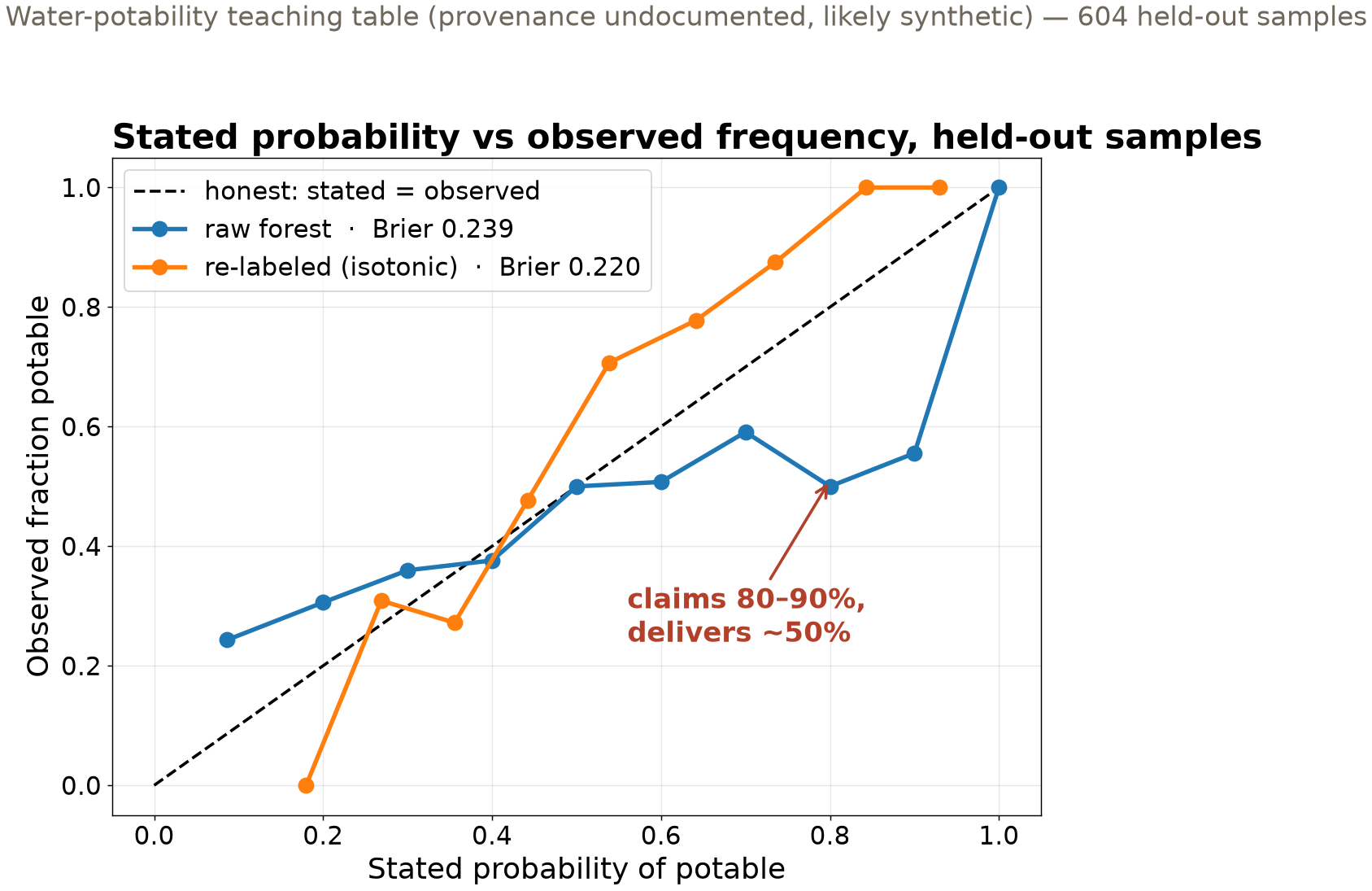
The overfit forest beats logistic on accuracy (0.62 vs 0.60) — and lies exactly where a user would act. Re-labeling repairs it: Brier 0.239 → 0.220.

The competitor: a small forest of 10 deep trees, each nearly memorizing the training set (training accuracy 0.974). Its “probability” is the fraction of trees voting potable — with 10 overfit trees, that lands on extreme values like 0.9 or 1.0. Read the blue curve: where the forest claims 80–90%, the observed frequency is ~50%. Test accuracy (0.619, better than logistic!) gives no hint — this is the slide’s punch: accuracy and honesty are different axes. The repair, in geoscience-first terms: hold samples out, record how often samples scored near 0.9 actually turn out potable, and re-label each score to that observed frequency — allowing only order-preserving corrections, so if the forest ranked A above B, corrected A stays at or above corrected B. The ranking survives; the numbers attached to it become honest. Result: Brier 0.239 → 0.220, and accuracy rises to 0.664 (partly a small ensemble bonus from averaging refits — not the point). Implementation names for the notebook: scikit-learn calls the order-preserving fit isotonic regression, wrapped in CalibratedClassifierCV with rotating held-out folds — the 3.8 idea, already at work.

The probability is the deliverable

• A geotechnical engineer reports probability of liquefaction → enters a building-code check
• A water manager acts on probability of a harmful algal bloom
• A floodplain map encodes probability of flood exceedance

The threshold owner is not the model trainer — they take your number at face value.

A miscalibrated 90% that means 55% silently moves your modeling error into someone else’s decision.

Slow down here; this is the “why” of the whole session. In each example the person who sets the decision threshold — how much probability justifies the cost of acting — is downstream: a code official, an operations manager, an insurer. They cannot see your training curves; they see the number. So the reporting standard follows: whenever your model’s probabilities feed a threshold you do not own, a reliability diagram and a Brier score belong next to the accuracy, as routinely as error bars belong on a measurement. Connect back to Brier 1950 — weather forecasting institutionalized exactly this discipline, and “there is a 70% chance of rain” means something because of it. Connect forward: ensemble disagreement gives a complementary uncertainty view on Friday (3.9), and lesson 4.5 runs this same reliability check on deep ensembles.

What we built today

Tool	The question it answers	Today’s answer
Baseline + held-out score	is there signal at all	0.598 vs 0.597 floor — barely
Gradient descent + autodiff	how every model in Ch. 4 learns	loss falls, gradients match calculus
Reliability diagram	does stated 80% happen 80% of the time	forest: no — delivers ~50%
Brier score + re-labeling	how wrong, and can it be repaired	0.239 → 0.220, ranking preserved

Two honest deliverables: a probability that means what it says, and a report that shows you checked.

Leave the table up for questions. Row by row: the near-null result is a feature of honest evaluation, not a failure; the opened box is the training loop the rest of the course reuses; the reliability diagram is the lie detector; the Brier-scored repair is the fix that preserves what the model ranked well. If one sentence survives the week, make it the takeaway of the previous slide: the threshold owner is not the model trainer.

Now run it yourself — open 3.6

1. pixi run jupyter lab → 3.6_logistic_regression.ipynb
2. Verify autodiff: run the one-observation cells — PyTorch’s gradients vs your calculus
3. Train the loop (torch.optim.SGD), then score: baseline, train, test
4. Calibrate: reliability diagrams and Brier scores; repair the forest with CalibratedClassifierCV(method='isotonic')

HW-CML assigned today, due Fri Nov 20 · Fri: trees, forests, ensembles (3.7 + 3.9) · leaderboard open through Nov 24

Timing for the 80-minute block (10:00–11:20): pulse talks ~10 min, deck ~20 min, notebook ~40 min, synthesis ~10 min. In the exercise, task 2 is where the box-opening becomes real — insist students compare the printed gradient values to the formulas, not just run the cells. Task 4 misconception to circulate for: students expect calibration to raise accuracy; say plainly that the repair targets the probabilities, and the small accuracy gain here is an ensemble side effect. HW-CML goes out today: rock-lithology classification on a synthetic geochemistry survey (mlgeo_synth, hidden-seed variant for spot checks) — data prep through model comparison and feature importance, so this week’s lessons are its toolkit. Synthesis question: in your project, who owns the decision threshold — you, or someone downstream? Collect three answers aloud; they seed the check-in on Nov 16.