Model Testing and Evaluation#
The goal of predicting Snow Water Equivalent exemplifies the integration of Machine learning with environmental science. This chapter delved into the testing and Evaluation part of this project.
Within the extensive array of functionalities provided by the BaseHole class, the testing process is akin to a rigorous examination.
8.1 Testing#
8.1.1 So, what is a test?#
The test function operates on a simple yet profound principle: it utilizes the model to predict outcomes based on the test dataset which the model has not seen earlier during the training. This method is fundamental to understanding how well the model generalizes to new, unseen data.
def test(self):
  '''
  Tests the machine learning model on the testing data.
  Returns: numpy.ndarray: The predicted results on the testing data.
  '''
  self.test_y_results = self.classifier.predict(self.test_x)
  return self.test_y_results
8.1.2. The Mechanic of Testing#
The test() method uses the trained model to make predictions on test_x, a dataset that was not part of the training process. The output, test_y_results, provides a preview of the model’s performance, offering insights into its predictive capabilities.
8.2 Validation/Evaluation#
8.2.1 Importance of Evaluation#
So now we have made a model, trained the model, and made predictions on a test dataset, but how to evaluate all of this?
For this, we use multiple Evaluation metrics. A model needs to go through a rigorous validation process that assesses its effectiveness and accuracy. Evaluation is a testament to the model’s commitment to precision, ensuring that the predictions made are not only reliable but also meaningful.
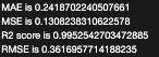
For this project we have a comprehensive suite of metrics – Mean Absolute Error (MAE), Mean Squared Error (MSE), R-squared (R2), and Root Mean Squared Error (RMSE). Each metric offers a unique lens through which the model’s performance can be scrutinized, from the average error per prediction (MAE) to the proportion of variance explained (R2).
8.2.2 Insights#
Upon invoking the evaluation method, the class starts a detailed analysis of the model’s predictions. By comparing these predictions against actual values from the test dataset, the method illuminates the model’s strengths and areas for improvement.
The output—a dictionary of metrics—serves as a beacon, guiding further refinement and optimization of the model.
The Testament of Metrics
MAE: This metric provides an average of the absolute errors between predicted and actual values, offering a straightforward measure of prediction accuracy.
MSE: By squaring the errors before averaging, MSE penalizes larger errors more heavily, providing insight into the variance of the model’s predictions.
R2: The R2 score reveals how well the model’s predictions conform to the actual data, serving as a gauge of the model’s explanatory power.
RMSE: As the square root of MSE, RMSE offers a measure of error in the same units as the predicted value, making it intuitively interpretable.
8.2.3 The Evaluation Process#
The evaluate() method in the model classes is responsible for computing the above metrics, using the predictions generated by the model and comparing them against actual values from the test dataset.
from sklearn.ensemble import RandomForestRegressor
import numpy as np
import pandas as pd
import matplotlib.pyplot as plt
import seaborn as sns
from sklearn.model_selection import train_test_split
from sklearn.preprocessing import MinMaxScaler
from sklearn.metrics import mean_squared_error
from sklearn import metrics
from sklearn import tree
import joblib
import os
from pathlib import Path
import json
# import geopandas as gpd
# import geojson
import os.path
import math
from sklearn.model_selection import RandomizedSearchCV

exit(0)  # for now, the workflow is not ready yet

# read the grid geometry file


# read the grid geometry file
homedir = os.path.expanduser('~')
print(homedir)
github_dir = f"{homedir}/Documents/GitHub/SnowCast"
modis_test_ready_file = f"{github_dir}/data/ready_for_training/modis_test_ready.csv"
modis_test_ready_pd = pd.read_csv(modis_test_ready_file, header=0, index_col=0)

pd_to_clean = modis_test_ready_pd[["year", "m", "doy", "ndsi", "swe", "station_id", "cell_id"]].dropna()

all_features = pd_to_clean[["year", "m", "doy", "ndsi"]].to_numpy()
all_labels = pd_to_clean[["swe"]].to_numpy().ravel()
def evaluate(self):
    y_predicted = model.predict(test_features)
    mae = metrics.mean_absolute_error(y_test, y_predicted)
    mse = metrics.mean_squared_error(y_test, y_predicted)
    r2 = metrics.r2_score(y_test, y_predicted)
    rmse = math.sqrt(mse)

    print("The {} model performance for testing set".format(model_name))
    print("--------------------------------------")
    print('MAE is {}'.format(mae))
    print('MSE is {}'.format(mse))
    print('R2 score is {}'.format(r2))
    print('RMSE is {}'.format(rmse))

    return y_predicted
Computing the Metrics: Leveraging the metrics module from scikit-learn, the function calculates MAE, MSE, R2, and RMSE. Each of these calculations provides a different lens through which to view the model’s performance, from average error rates (MAE, RMSE) to the model’s explanatory power (R2) and the variance of its predictions (MSE).
Interpreting the Results: The function not only computes these metrics but also prints them out, offering immediate insight into the model’s efficacy. This step is vital for iterative model improvement, allowing data scientists to diagnose and address specific areas where the model may fall short.
Returning the Metrics: Finally, the function encapsulates these metrics in a dictionary and returns it. This encapsulation allows for the metrics to be easily accessed, shared, and utilized in further analyses or reports, facilitating a deeper understanding of the model’s impact and areas for enhancement.
8.2.4 Practical Example of Evaluation#
The script provides practical examples by loading pre-trained models and evaluating them using the test dataset:
base_model = joblib.load(f"{homedir}/Documents/GitHub/snowcast_trained_model/model/wormhole_random_forest_basic.joblib")
basic_predicted_values = evaluate(base_model, all_features, all_labels, "Base Model")

best_random = joblib.load(f"{homedir}/Documents/GitHub/snowcast_trained_model/model/wormhole_random_forest.joblib")
random_predicted_values = evaluate(best_random, all_features, all_labels, "Optimized")
Here, the script loads two models—a base model and an optimized model—and evaluates their performance on the same test dataset. This side-by-side comparison allows for an assessment of how model optimization impacts predictive accuracy and overall performance.
Testing and validation form the bedrock of predictive excellence in the SnowCast project. They are not merely steps in the machine learning workflow but are essential processes that ensure the models we build are reliable interpreters of environmental data. By rigorously testing and evaluating models, we can trust that their predictions will be both accurate and meaningful in real-world applications.