Model Prediction/Evaluation#
Finally, we are at the final Chapter where we see the end-product of the model created. As we venture into this critical phase, the model_predict script emerges, guiding the way toward understanding and anticipating the future of snow water equivalent (SWE) through the ExtraTree model. This chapter delves into the intricacies of this script, unraveling the processes that transforms raw, unprocessed data into precise predictions that illuminate the path forward.
import joblib
import pandas as pd
from sklearn.preprocessing import MinMaxScaler, StandardScaler
import numpy as np
import os
import random
import string
import shutil


def generate_random_string(length):
    # Define the characters that can be used in the random string
    characters = string.ascii_letters + string.digits  # You can customize this to include other characters if needed

    # Generate a random string of the specified length
    random_string = ''.join(random.choice(characters) for _ in range(length))

    return random_string
homedir = os.path.expanduser('~')
work_dir = f"{homedir}/gridmet_test_run"

test_start_date = ''

selected_columns = [
  'swe_value',
  'SWE',
  'cumulative_SWE',
#   'cumulative_relative_humidity_rmin',
#   'cumulative_air_temperature_tmmx',
#   'cumulative_air_temperature_tmmn',
#   'cumulative_relative_humidity_rmax',
#   'cumulative_potential_evapotranspiration',
#   'cumulative_wind_speed',
  #'cumulative_fsca',
  'fsca',
  'air_temperature_tmmx',
  'air_temperature_tmmn',
  'potential_evapotranspiration',
  'relative_humidity_rmax',
  'Elevation',
  'Slope',
  'Curvature',
  'Aspect',
  'Eastness',
  'Northness',
]


def month_to_season(month):
    if 3 <= month <= 5:
        return 1
    elif 6 <= month <= 8:
        return 2
    elif 9 <= month <= 11:
        return 3
    else:
        return 4
9.1 Data Loading and Preprocessing#
9.1.1 Loading the Data#
The prediction process begins with loading of data from a CSV file. This data includes a vast array of variables that are essential for making accurate SWE predictions.
def load_data(file_path):
  """
  Load data from a CSV file.
  Args: file_path (str): Path to the CSV file containing the data.
  Returns: pd.DataFrame: A pandas DataFrame containing the loaded data.
   """
  return pd.read_csv(file_path)
9.1.2 Preprocessing the Data#
Once loaded, the data undergoes a transformation process to ensure it aligns with the model’s requirements. This step includes converting dates, renaming columns for consistency, and selecting relevant features.
Prepprocessing is crucial to ensure that the data is in the correct format for the model, which directly impacts the accurancy of the prefictions.
def preprocess_data(data):
  """
  Preprocess the input data for model prediction.
  Args: data (pd.DataFrame): Input data in the form of a pandas DataFrame.
  Returns: pd.DataFrame: Preprocessed data ready for prediction.
  """
  data['date'] = pd.to_datetime(data['date'])
  data.replace('--', pd.NA, inplace=True)
  data.rename(columns={'Latitude': 'lat', 'Longitude': 'lon',
                       'vpd': 'mean_vapor_pressure_deficit',
                       'vs': 'wind_speed', 'pr': 'precipitation_amount',
                       'etr': 'potential_evapotranspiration', 'tmmn': 'air_temperature_tmmn',
                       'tmmx': 'air_temperature_tmmx', 'rmin': 'relative_humidity_rmin',
                       'rmax': 'relative_humidity_rmax', 'cumulative_AMSR_SWE': 'cumulative_SWE',
                       'cumulative_AMSR_Flag': 'cumulative_Flag', 'cumulative_tmmn':'cumulative_air_temperature_tmmn',
                       'cumulative_etr': 'cumulative_potential_evapotranspiration', 'cumulative_vpd': 'cumulative_mean_vapor_pressure_deficit',
                       'cumulative_rmax': 'cumulative_relative_humidity_rmax', 'cumulative_rmin': 'cumulative_relative_humidity_rmin',
                       'cumulative_pr': 'cumulative_precipitation_amount', 'cumulative_tmmx': 'cumulative_air_temperature_tmmx',
                       'cumulative_vs': 'cumulative_wind_speed', 'AMSR_SWE': 'SWE', 'AMSR_Flag': 'Flag', }, inplace=True)
  print(data.head())
  print(data.columns)
  selected_columns.remove("swe_value")
  desired_order = selected_columns + ['lat', 'lon',]
  data = data[desired_order]
  data = data.reindex(columns=desired_order)
  print("reorganized columns: ", data.columns)
  return data
9.2 Model Loading and Prediction#
9.2.1 Loading the Model#
The script retrieves the pre-trained ExtraTree model, which is used to generate predictions based on the processed data.
def load_model(model_path):
    """
    Load a machine learning model from a file.

    Args:
        model_path (str): Path to the saved model file.

    Returns:
        model: The loaded machine learning model.
    """
    return joblib.load(model_path)
9.2.2 Predicting SWE#
The predict_swe function prepares the input data and generates predictions using the loaded model.
def predict_swe(model, data):
  """
  Predict snow water equivalent (SWE) using a machine learning model.
  Args: model: The machine learning model for prediction.
  data (pd.DataFrame): Input data for prediction.
  Returns: pd.DataFrame: Dataframe with predicted SWE values.
  """
  data = data.fillna(-999)
  input_data = data
  input_data = data.drop(["lat", "lon"], axis=1)
  predictions = model.predict(input_data)
  data['predicted_swe'] = predictions
  return data
It fills missing values with a designated placeholder (-999), a common practice to ensure machine learning algorithms, can process the data without encountering errors due to missing values. This step reflects a balance between data integrity and computational requirements, enabling the model to make predictions even in the absence of complete information.
At the core of predict_swe is the model’s
predict()method invocation. This step is where the machine learning model, trained on historical data, applies its learned patterns to the new, unseen data. The decision to drop geographical identifiers (lat, lon) before prediction underscores a focus on the environmental and temporal factors influencing SWE, aligning the model’s inputs with its training regime.The function concludes by appending the model’s predictions back to the original dataset as a new column,
predicted_swe. This enrichment transforms the dataset from a static snapshot of past and present conditions into a dynamic forecast of future snow water equivalents. This step is critical for stakeholders relying on accurate SWE predictions.
9.2.3 Predict Function#
The predict function is what manages the entire prediction process from start to finish. It starts by loading the pre-trained model, which embodies the project’s strength of making predictions by preserving and leveraging the accumulated knowledge encapsulated within the model’s parameters.
def predict():
    """
    Main function for predicting snow water equivalent (SWE).
    Returns: None
    """
    height = 666
    width = 694
    model_path = f'{homedir}/Documents/GitHub/SnowCast/model/wormhole_ETHole_latest.joblib'
    print(f"Using model: {model_path}")

    new_data_path = f'{work_dir}/testing_all_ready_{test_start_date}.csv'
    latest_output_path = f'{work_dir}/test_data_predicted_latest_{test_start_date}.csv'
    output_path = f'{work_dir}/test_data_predicted_{generate_random_string(5)}.csv'

    if os.path.exists(output_path):
        os.remove(output_path)
        print(f"File '{output_path}' has been removed.")

    model = load_model(model_path)
    new_data = load_data(new_data_path)
    #print("new_data shape: ", new_data.head())

    preprocessed_data = preprocess_data(new_data)
    if len(new_data) < len(preprocessed_data):
      raise ValueError("Why the preprocessed data increased?")

    predicted_data = predict_swe(model, preprocessed_data)
    print("how many predicted? ", len(predicted_data))

    if "date" not in preprocessed_data:
      preprocessed_data["date"] = test_start_date
    predicted_data = merge_data(preprocessed_data, predicted_data)

    predicted_data.to_csv(output_path, index=False)
    print("Prediction successfully done ", output_path)

    shutil.copy(output_path, latest_output_path)
    print(f"Copied to {latest_output_path}")
Following model loading, the function navigates the data landscape, loading new data for prediction and preprocessing it to align with the model’s requirements. This step is critical, as it transforms raw data into a format that the model can interpret, ensuring the accuracy and relevance of the predictions.
9.3 Post-Processing and Merging Data#
9.3.1 Merging Predicted Data#
merge_data meticulously combines the predicted SWE values with the original dataset. It employs conditional logic to adjust predictions based on specific criteria, such as nullifying predictions in the absence of key environmental data. This approach underscores a commitment to precision, ensuring that the predictions reflect a nuanced understanding of the environmental context.
def merge_data(original_data, predicted_data):
"""
Merge predicted SWE data with the original data.
Args: original_data (pd.DataFrame): Original input data.
predicted_data (pd.DataFrame): Dataframe with predicted SWE values.
Returns: pd.DataFrame: Merged dataframe.
"""
if "date" not in predicted_data:
predicted_data["date"] = test_start_date
new_data_extracted = predicted_data[["date", "lat", "lon", "predicted_swe"]]
print("original_data.columns: ", original_data.columns)
print("new_data_extracted.columns: ", new_data_extracted.columns)
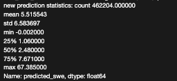
print("new prediction statistics: ", new_data_extracted["predicted_swe"].describe())
merged_df = original_data.merge(new_data_extracted, on=['date', 'lat', 'lon'], how='left')
merged_df.loc[merged_df['fsca'] == 237, 'predicted_swe'] = 0
merged_df.loc[merged_df['fsca'] == 239, 'predicted_swe'] = 0
merged_df.loc[merged_df['cumulative_fsca'] == 0, 'predicted_swe'] = 0
merged_df.loc[merged_df['air_temperature_tmmx'].isnull(), 'predicted_swe'] = 0
return merged_df
9.3.2 Technical Execution of the function#
Merging datasets based on date, latitude, and longitude—exemplifies the complex use of data science. It ensures that each predicted SWE value is accurately aligned with its corresponding geographical and temporal marker, preserving the integrity and utility of the predictions. This process not only highlights the technical sophistication of the SnowCast project but also its dedication to delivering reliable and actionable insights.
9.4 Delivering Predictions#
Finally, the predict function executes predict_swe, merges the predictions with the original data, and saves the enriched dataset. The choice of a dynamically generated filename for saving predictions demonstrates an understanding of operational requirements, ensuring that each prediction cycle is uniquely identifiable.
9.5 Results#
9.5.1 Converting the Predictions into Images#
These are the different functions used for this process of predicitons to Images
convert csvs to images simple: This Is the function that takes the raw data and converts them into Geographical images.
Data Loading: This begins by ingesting the CSV containing SWE predictions, ensuring every data point is primed for visualization.
Custom Colormap Creation: It employs a custom colormap, crafted to represent various ranges of SWE, providing an intuitive visual understanding of snow coverage.
Geospatial Plotting: This utilizes the geographical coordinates within the data to accurately place each prediction on the map, ensuring a realistic representation of SWE distribution.
Merge data: The merge_data function combines the predicted SWE values with their corresponding geographical markers.
Conditional Adjustments: Conditional adjustment refines the predicted values based on specific criteria, ensuring the visual representation aligns with realistic expectations of SWE.
Spatial Accuracy: This aligns predictions with their exact geographical locations, ensuring that the visual output is as informative as it is accurate.
Custom Colormap: A list named colors defines the color scheme for the colormap, using RGB tuples for each color. These colors are intended to represent different levels of SWE, from low to high(light gray to dark red).
Geographical Boundaries: lon_min, lon_max, lat_min, and lat_max define the geographical area of interest by specifying the minimum and maximum longitudes and latitudes. This setting targets the visualization and analysis efforts to the Western United States.
import matplotlib.colors as mcolors


colors = [
    (0.8627, 0.8627, 0.8627),  # #DCDCDC - 0 - 1
    (0.8627, 1.0000, 1.0000),  # #DCFFFF - 1 - 2
    (0.6000, 1.0000, 1.0000),  # #99FFFF - 2 - 4
    (0.5569, 0.8235, 1.0000),  # #8ED2FF - 4 - 6
    (0.4509, 0.6196, 0.8745),  # #739EDF - 6 - 8
    (0.4157, 0.4706, 1.0000),  # #6A78FF - 8 - 10
    (0.4235, 0.2784, 1.0000),  # #6C47FF - 10 - 12
    (0.5529, 0.0980, 1.0000),  # #8D19FF - 12 - 14
    (0.7333, 0.0000, 0.9176),  # #BB00EA - 14 - 16
    (0.8392, 0.0000, 0.7490),  # #D600BF - 16 - 18
    (0.7569, 0.0039, 0.4549),  # #C10074 - 18 - 20
    (0.6784, 0.0000, 0.1961),  # #AD0032 - 20 - 30
    (0.5020, 0.0000, 0.0000)   # #800000 - > 30
]
cmap_name = 'custom_snow_colormap'
custom_cmap = mcolors.ListedColormap(colors)

lon_min, lon_max = -125, -100
lat_min, lat_max = 25, 49.5

# Define value ranges for color mapping
fixed_value_ranges = [1, 2, 4, 6, 8, 10, 12, 14, 16, 18, 20, 30]
Convert csv to geotiff: This function mainly helps in converting images to geographically accurate maps.
Rasterization: It transforms the CSV data into a raster format, suitable for creating detailed geospatial maps.
Resolution and Coverage: This carefully defines the resolution and geographical extent of the output map, ensuring that it captures the full scope of the predictions.
Geospatial Alignment: Geospatial Alignment utilizes rasterio and geopandas libraries to ensure that each pixel in the output map accurately represents the predicted SWE values at specific geographical coordinates.
def convert_csvs_to_images():
    """
    Convert CSV data to images with color-coded SWE predictions.

    Returns:
        None
    """
    global fixed_value_ranges
    data = pd.read_csv(f"{homedir}/gridmet_test_run/test_data_predicted_n97KJ.csv")
    print("statistic of predicted_swe: ", data['predicted_swe'].describe())
    data['predicted_swe'].fillna(0, inplace=True)

    for column in data.columns:
        column_data = data[column]
        print(column_data.describe())

    # Create a figure with a white background
    fig = plt.figure(facecolor='white')


    m = Basemap(llcrnrlon=lon_min, llcrnrlat=lat_min, urcrnrlon=lon_max, urcrnrlat=lat_max,
                projection='merc', resolution='i')

    x, y = m(data['lon'].values, data['lat'].values)
    print(data.columns)

    color_mapping, value_ranges = create_color_maps_with_value_range(data["predicted_swe"], fixed_value_ranges)

    # Plot the data using the custom colormap
    plt.scatter(x, y, c=color_mapping, cmap=custom_cmap, s=30, edgecolors='none', alpha=0.7)

    # Draw coastlines and other map features
    m.drawcoastlines()
    m.drawcountries()
    m.drawstates()

    reference_date = datetime(1900, 1, 1)
    day_value = day_index

    result_date = reference_date + timedelta(days=day_value)
    today = result_date.strftime("%Y-%m-%d")
    timestamp_string = result_date.strftime("%Y-%m-%d")

    # Add a title
    plt.title(f'Predicted SWE in the Western US - {today}', pad=20)

    # Add labels for latitude and longitude on x and y axes with smaller font size
    plt.xlabel('Longitude', fontsize=6)
    plt.ylabel('Latitude', fontsize=6)

    # Add longitude values to the x-axis and adjust font size
    x_ticks_labels = np.arange(lon_min, lon_max + 5, 5)
    x_tick_labels_str = [f"{lon:.1f}°W" if lon < 0 else f"{lon:.1f}°E" for lon in x_ticks_labels]
    plt.xticks(*m(x_ticks_labels, [lat_min] * len(x_ticks_labels)), fontsize=6)
    plt.gca().set_xticklabels(x_tick_labels_str)

    # Add latitude values to the y-axis and adjust font size
    y_ticks_labels = np.arange(lat_min, lat_max + 5, 5)
    y_tick_labels_str = [f"{lat:.1f}°N" if lat >= 0 else f"{abs(lat):.1f}°S" for lat in y_ticks_labels]
    plt.yticks(*m([lon_min] * len(y_ticks_labels), y_ticks_labels), fontsize=6)
    plt.gca().set_yticklabels(y_tick_labels_str)

    # Convert map coordinates to latitude and longitude for y-axis labels
    y_tick_positions = np.linspace(lat_min, lat_max, len(y_ticks_labels))
    y_tick_positions_map_x, y_tick_positions_map_y = lat_lon_to_map_coordinates([lon_min] * len(y_ticks_labels), y_tick_positions, m)
    y_tick_positions_lat, _ = m(y_tick_positions_map_x, y_tick_positions_map_y, inverse=True)
    y_tick_positions_lat_str = [f"{lat:.1f}°N" if lat >= 0 else f"{abs(lat):.1f}°S" for lat in y_tick_positions_lat]
    plt.yticks(y_tick_positions_map_y, y_tick_positions_lat_str, fontsize=6)

    # Create custom legend elements using the same colormap
    legend_elements = [Patch(color=colors[i], label=f"{value_ranges[i]} - {value_ranges[i+1]-1}" if i < len(value_ranges) - 1 else f"> {value_ranges[-1]}") for i in range(len(value_ranges))]

    # Create the legend outside the map
    legend = plt.legend(handles=legend_elements, loc='upper left', title='Legend', fontsize=8)
    legend.set_bbox_to_anchor((1.01, 1))

    # Remove the color bar
    #plt.colorbar().remove()

    plt.text(0.98, 0.02, 'Copyright © SWE Wormhole Team',
             horizontalalignment='right', verticalalignment='bottom',
             transform=plt.gcf().transFigure, fontsize=6, color='black')

    # Set the aspect ratio to 'equal' to keep the plot at the center
    plt.gca().set_aspect('equal', adjustable='box')

    # Adjust the bottom and top margins to create more white space between the title and the plot
    plt.subplots_adjust(bottom=0.15, right=0.80)  # Adjust right margin to accommodate the legend
    # Show the plot or save it to a file
    new_plot_path = f'{homedir}/gridmet_test_run/predicted_swe-{test_start_date}.png'
    print(f"The new plot is saved to {new_plot_path}")
    plt.savefig(new_plot_path)
    # plt.show()  # Uncomment this line if you want to display the plot directly instead of saving it to a file
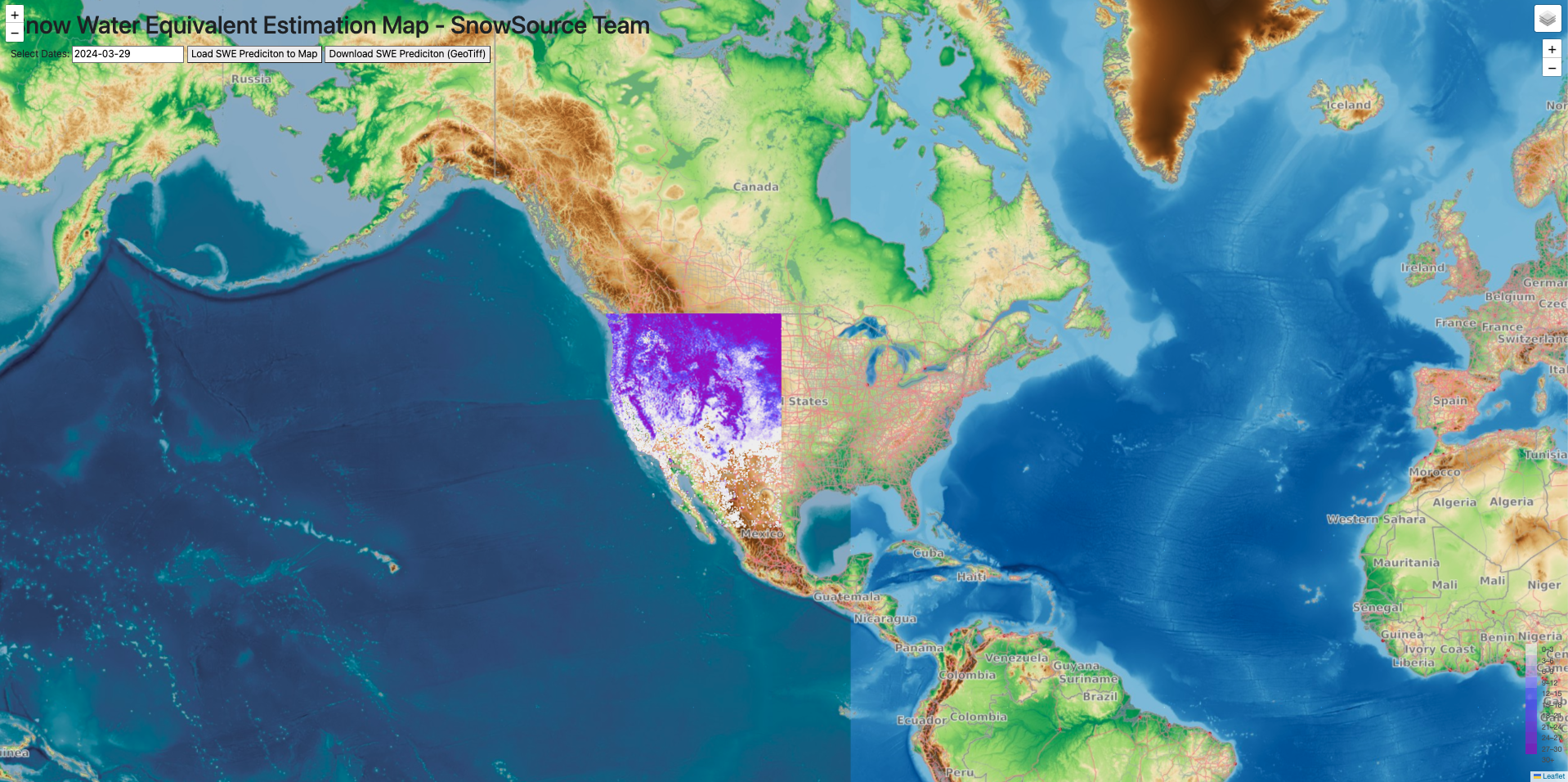
9.5.2 Deploy images to website#
This is the process that helps in Deploying the visual insights
1. copy files to right folder –
Function: Bridging Computational Outputs with Public Access At the heart of our deployment strategy lies the copy_files_to_right_folder function. This function acts as the bridge, transferring the visual and data outputs of SnowCast from the secure confines of its computational environment to a publicly accessible web directory.
Here’s how it achieves this pivotal role:
Folder Synchronization: Utilizing distutils.dir_util.copy_tree, it ensures that all visual comparisons and predictions are mirrored from the SnowCast workspace to the web server’s plotting directory, maintaining up-to-date access for users worldwide.
Selective Deployment: Through meticulous directory traversal, it distinguishes between .png visualizations and .tif geospatial files, ensuring each file type is deployed to its rightful place for optimal public utility.
2. create mapserver map config: Crafts interactive Maps
The magic of SnowCast is not just in its predictions but in how these predictions are presented. The create_mapserver_map_config function crafts a MapServer configuration for each GeoTIFF prediction file, transforming static data into interactive, exploratory maps.
Dynamic Configuration: By generating a .map file for each prediction, this function lays the groundwork for interactive map services, allowing users to explore SWE predictions across different regions and times.
Intuitive Visualization: The custom MapServer configuration leverages the power of geographical information systems (GIS) to provide an intuitive, visual representation of complex SWE data, making it accessible to experts and laypeople alike.
3. refresh available date list: Refreshing the Forecast
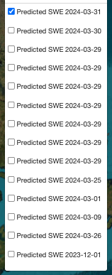
The refresh_available_date_list function ensures that the SnowCast portal remains current, reflecting the latest predictions and analyses. By dynamically updating the available date list with new predictions, it guarantees that users have access to the most recent insights.
Data Frame Dynamics: This function creates a pandas DataFrame to catalog the available predictions, linking each date with its corresponding visualization and data file, thereby ensuring the portal’s content is both comprehensive and current.
Seamless Integration: The updated date list is saved as a CSV file, seamlessly integrating with the web portal’s infrastructure to refresh the interactive calendar, guiding users to the latest SWE predictions.