Cumulative Time Series Analysis#
In this chapter we process and analyze Snow Water Equivalent (SWE) and meteorological data to prepare it for time series analysis.
This transformation is essential for analyzing how specific variables, such as
snow coverandtemperature, change over time at different geographic locations.
5.1 Importing the libraries and Input files#
Here we set up the environment and define file paths for managing and processing environmental data.
Dask is a parallel computing library in Python that enables scalable and distributed computing.
current_ready_csv_pathholds the file path for the initial dataset that has been merged and sorted. The dataset contains data from the past three years and includes all active stations.cleaned_csv_pathdefines the path for a cleaned version of the dataset.target_time_series_csv_pathspecifies the file path where the time series version of the cleaned dataset will be saved.backup_time_series_csv_pathholds the file path for a backup of the time series dataset.target_time_series_cumulative_csv_pathdefines the file path for a cumulative version of the time series dataset.
#Importing the required libraries
import pandas as pd
import os
import shutil
import numpy as np
import dask.dataframe as dd

homedir = os.path.expanduser('~')
work_dir = f"../data"

# Set Pandas options to display all columns
pd.set_option('display.max_columns', None)


# Define file paths for various CSV files
current_ready_csv_path = f'{work_dir}/final_merged_data_3yrs_all_active_stations_v1.csv_sorted.csv'
cleaned_csv_path = f"{current_ready_csv_path}_cleaned_nodata.csv"
target_time_series_csv_path = f'{cleaned_csv_path}_time_series_v1.csv'
backup_time_series_csv_path = f'{cleaned_csv_path}_time_series_v1_bak.csv'
target_time_series_cumulative_csv_path = f'{cleaned_csv_path}_time_series_cumulative_v1.csv'
5.2 Cleaning and Preparation#
Here we clean the dataset to remove rows with missing SWE values. We Utilize Dask for efficient processing of potentially large datasets, ensuring scalability and performance.
def clean_non_swe_rows(current_ready_csv_path, cleaned_csv_path):
    # Read Dask DataFrame from CSV
    dask_df = dd.read_csv(current_ready_csv_path, dtype={'stationTriplet': 'object',
       'station_name': 'object'})

    # Remove rows where 'swe_value' is empty
    dask_df_filtered = dask_df.dropna(subset=['swe_value'])

    # Save the result to a new CSV file
    dask_df_filtered.to_csv(cleaned_csv_path, index=False, single_file=True)
    print("dask_df_filtered.shape = ", dask_df_filtered.shape)
    print(f"The filtered csv with no swe values is saved to {cleaned_csv_path}")

clean_non_swe_rows(current_ready_csv_path, cleaned_csv_path)
dask_df_filtered.shape =  (Delayed('int-5cc8b7ae-25d5-478c-b53d-664926e9ce4f'), 26)
The filtered csv with no swe values is saved to ../data/final_merged_data_3yrs_all_active_stations_v1.csv_sorted.csv_cleaned_nodata.csv
5.3 Interpolation and Missing Data Handling#
With a clean dataset, we proceed to interpolate missing values for specified columns.
We perform in-place interpolation of missing values for specified columns, using a polynomial of a given degree.
We check for specific conditions (e.g., SWE values above a certain threshold) to decide on the interpolation strategy. It ensures that no null values remain post-interpolation, maintaining the dataset’s completeness.
x = df.index: Represents the index of the DataFrame.y = df[column_name]: Represents the values of the specified column (column_name) in the DataFrame.
def interpolate_missing_inplace(df, column_name, degree=3):
    x = df.index
    y = df[column_name]

    # Create a mask for missing values
    if column_name == "SWE":
      mask = (y > 240) | y.isnull()
    elif column_name == "fsca":
      mask = (y > 100) | y.isnull()
    else:
      mask = y.isnull()

    # Check if all elements in the mask array are True
    all_true = np.all(mask)

    if all_true:
      df[column_name] = 0
    else:
      # Perform interpolation
      new_y = np.interp(x, x[~mask], y[~mask])
      # Replace missing values with interpolated values
      df[column_name] = new_y

    if np.any(df[column_name].isnull()):
      raise ValueError("Single group: shouldn't have null values here")

    return df
5.4 Conversion to Time Series Format#
Next, we convert the dataset into a time series format.
We transform the dataset into a time series format, sorting data and filling missing values with interpolated data.
We then read the cleaned CSV, sorts the data, performs interpolation for missing values, and structures the dataset for time series analysis.
columns_to_be_time_series = ["SWE",
                                 'air_temperature_tmmn',
                                 'potential_evapotranspiration',
                                 'mean_vapor_pressure_deficit',
                                 'relative_humidity_rmax',
                                 'relative_humidity_rmin',
                                 'precipitation_amount',
                                 'air_temperature_tmmx',
                                 'wind_speed',
                                 'fsca']

# Read the cleaned ready CSV
df = pd.read_csv(cleaned_csv_path)
df.sort_values(by=['lat', 'lon', 'date'], inplace=True)
print("All current columns: ", df.columns)

    # rename all columns to unified names
    #     ['date', 'lat', 'lon', 'SWE', 'Flag', 'swe_value', 'cell_id',
# 'station_id', 'etr', 'pr', 'rmax', 'rmin', 'tmmn', 'tmmx', 'vpd', 'vs',
# 'elevation', 'slope', 'curvature', 'aspect', 'eastness', 'northness',
# 'fsca']
df.rename(columns={'vpd': 'mean_vapor_pressure_deficit',
                        'vs': 'wind_speed',
                        'pr': 'precipitation_amount',
                        'etr': 'potential_evapotranspiration',
                        'tmmn': 'air_temperature_tmmn',
                        'tmmx': 'air_temperature_tmmx',
                        'rmin': 'relative_humidity_rmin',
                        'rmax': 'relative_humidity_rmax',
                        'AMSR_SWE': 'SWE',
                        'fSCA': 'fsca'
                    }, inplace=True)

filled_csv = f"{target_time_series_csv_path}_gap_filled.csv"
All current columns:  Index(['date', 'lat', 'lon', 'AMSR_SWE', 'station_name', 'swe_value',
       'change_in_swe_inch', 'snow_depth', 'air_temperature_observed_f',
       'air_temperature_tmmn', 'potential_evapotranspiration',
       'mean_vapor_pressure_deficit', 'relative_humidity_rmax',
       'relative_humidity_rmin', 'precipitation_amount',
       'air_temperature_tmmx', 'wind_speed', 'stationTriplet', 'elevation',
       'Elevation', 'Slope', 'Aspect', 'Curvature', 'Northness', 'Eastness',
       'fSCA'],
      dtype='object')
5.5 Handling Missing Data and Interpolation#
Here we handle missing data within a dataset by using polynomial interpolation.
process_group_filling_value(group)is defined to handle the interpolation for each group of data, sorted by date. It goes through each relevant column (columns_to_be_time_series) and fills in the missing values using interpolation.The data is then grouped by geographic coordinates (
lat,lon) to apply the interpolation within each group.
if os.path.exists(filled_csv):
        print(f"{filled_csv} already exists, skipping")
        filled_data = pd.read_csv(filled_csv)
else:
    # Function to perform polynomial interpolation and fill in missing values
    def process_group_filling_value(group):
        # Sort the group by 'date'
        group = group.sort_values(by='date')

        for column_name in columns_to_be_time_series:
            group = interpolate_missing_inplace(group, column_name)
        # Return the processed group
        return group
    # Group the data by 'lat' and 'lon' and apply interpolation for each column
    print("Start to fill in the missing values")
    grouped = df.groupby(['lat', 'lon'])
    filled_data = grouped.apply(process_group_filling_value).reset_index(drop=True)


    if any(filled_data['fsca'] > 100):
        raise ValueError("Error: shouldn't have SWE>240 at this point")

    filled_data.to_csv(filled_csv, index=False)

    print(f"New filled values csv is saved to {filled_csv}")
../data/final_merged_data_3yrs_all_active_stations_v1.csv_sorted.csv_cleaned_nodata.csv_time_series_v1.csv_gap_filled.csv already exists, skipping
5.6 Creating Time Series Data with Previous 7 Days’ Values#
Here we generate a new CSV file containing time series data, where each location’s data is augmented with columns representing the previous 7 days’ values. If the file already exists, it skips the process.
process_group_time_seriesis to handle the creation of time series columns for each location group.For each group, the data is sorted by
date.Then we iterate through the previous 7 days (
num_days = 7), creating new columns for each target variable (columns_to_be_time_series), with the suffix_dayrepresenting how many days back the data is from.
if os.path.exists(target_time_series_csv_path):
        print(f"{target_time_series_csv_path} already exists, skipping")
else:
    df = filled_data
    # Create a new DataFrame to store the time series data for each location
    print("Start to create the training csv with previous 7 days columns")
    result = pd.DataFrame()

    # Define the number of days to consider (7 days in this case)
    num_days = 7

    grouped = df.groupby(['lat', 'lon'])

    def process_group_time_series(group, num_days):
        group = group.sort_values(by='date')
        for day in range(1, num_days + 1):
            for target_col in columns_to_be_time_series:
                new_column_name = f'{target_col}_{day}'
                group[new_column_name] = group[target_col].shift(day)

        return group

    result = grouped.apply(lambda group: process_group_time_series(group, num_days)).reset_index(drop=True)
    result.fillna(0, inplace=True)

    result.to_csv(target_time_series_csv_path, index=False)
    print(f"New data is saved to {target_time_series_csv_path}")
    shutil.copy(target_time_series_csv_path, backup_time_series_csv_path)
    print(f"File is backed up to {backup_time_series_csv_path}")
../data/final_merged_data_3yrs_all_active_stations_v1.csv_sorted.csv_cleaned_nodata.csv_time_series_v1.csv already exists, skipping
5.7 Addition of Cumulative Columns#
Here we add cumulative columns for specific variables. We take a CSV file containing time series data and adds cumulative columns for specific variables. And then save the processed data to a new CSV file and generates plots for the cumulative variables.
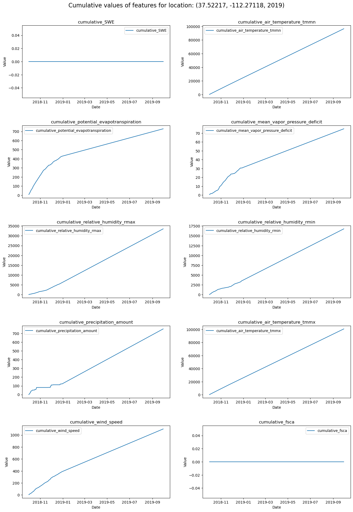
Here we calculate cumulative values for certain climate-related variables over time and visualize the cumulative trends for a specific location.
input_csvThe path to the input CSV file containing the time series data.output_csv: The path to the output CSV file where the cumulative data will be saved.force: A boolean flag to force the operation (even though it is defined, it is not explicitly used in the code).Calculate Water Year:A water year starts on October 1st and ends on September 30th of the next year.
The function calculates the water year for each row and adds it as a new column.
The data is grouped by latitude (
lat), longitude (lon), and water year.For each variable listed in
columns_to_be_cumulated, a cumulative column is added to the DataFrame.The cumulative value is calculated using the
cumsum()function within each group.
Example Variables#
SWE: Snow Water Equivalentair_temperature_tmmn: Minimum air temperaturepotential_evapotranspiration: Potential evapotranspirationmean_vapor_pressure_deficit: Mean vapor pressure deficitrelative_humidity_rmax: Maximum relative humidityrelative_humidity_rmin: Minimum relative humidityprecipitation_amount: Amount of precipitationair_temperature_tmmx: Maximum air temperaturewind_speed: Wind speedfsca: Fractional snow-covered areaThe addition of cumulative columns to the dataset offers a dynamic perspective on environmental time series data. By aggregating measurements such as temperature, precipitation, and wind speed, the function reveals the incremental changes and long-term accumulation of these factors over specific periods – particularly water years. This comprehensive view is instrumental in understanding trends and patterns that are not immediately apparent in daily or monthly data.
import pandas as pd
import seaborn as sns
import matplotlib.pyplot as plt
import numpy as np
def add_cumulative_columns(input_csv, output_csv, force=False):
    """
    Add cumulative columns to the time series dataset.

    This function reads the time series CSV file created by `convert_to_time_series`, calculates cumulative values for specific columns, and saves the data to a new CSV file.
    """

    columns_to_be_cumulated = [
      "SWE",
      'air_temperature_tmmn',
      'potential_evapotranspiration',
      'mean_vapor_pressure_deficit',
      'relative_humidity_rmax',
      'relative_humidity_rmin',
      'precipitation_amount',
      'air_temperature_tmmx',
      'wind_speed',
      'fsca'
    ]

    # Read the time series CSV (ensure it was created using `convert_to_time_series` function)
    # directly read from original file
    df = pd.read_csv(input_csv)

    print("The column statistics from time series before cumulative: ", df.describe()),

    df['date'] = pd.to_datetime(df['date'])

    unique_years = df['date'].dt.year.unique()
    print("This is our unique years", unique_years)
    #current_df['fSCA'] = current_df['fSCA'].fillna(0)

    # only start from the water year 10-01
    # Filter rows based on the date range (2019 to 2022)
    start_date = pd.to_datetime('2018-10-01')
    end_date = pd.to_datetime('2021-09-30')
    df = df[(df['date'] >= start_date) & (df['date'] <= end_date)]
    print("how many rows are left in the three water years?", len(df.index))
    df.to_csv(f"{current_ready_csv_path}.test_check.csv")

    # Define a function to calculate the water year
    def calculate_water_year(date):
        year = date.year
        if date.month >= 10:  # Water year starts in October
            return year + 1
        else:
            return year

    # every water year starts at Oct 1, and ends at Sep 30.
    df['water_year'] = df['date'].apply(calculate_water_year)

    # Group the DataFrame by 'lat' and 'lon'
    grouped = df.groupby(['lat', 'lon', 'water_year'], group_keys=False)
    print("how many groups? ", len(grouped))

    # grouped = df.groupby(['lat', 'lon', 'water_year'], group_keys=False)
    for column in columns_to_be_cumulated:
        df[f'cumulative_{column}'] = grouped.apply(lambda group: group.sort_values('date')[column].cumsum())

    print("This is the dataframe after cumulative columns are added")
    print(df.columns)

    df.to_csv(output_csv, index=False)

    print(f"All the cumulative variables are added successfully! {target_time_series_cumulative_csv_path}")
    print("double check the swe_value statistics:", df["swe_value"].describe())
    cumulative_columns = [f'cumulative_{col}' for col in columns_to_be_cumulated]
    # Number of rows and columns for subplots
    n_rows = len(cumulative_columns) // 2
    n_cols = 2
    # Create subplots
    fig, axes = plt.subplots(n_rows, n_cols, figsize=(14, n_rows * 4))

    # Flatten axes array if more than one row
    if n_rows > 1:
        axes = axes.flatten()

    first_group_name = list(grouped.groups.keys())[0]

    # Get the first group
    first_group = grouped.get_group(first_group_name)

    print("-------------------------")
    print(first_group)

    # Plot each cumulative column in a subplot
    for i, col in enumerate(cumulative_columns):
        axes[i].plot(first_group['date'], first_group[col], label=col)
        axes[i].set_title(col)
        axes[i].set_xlabel('Date')
        axes[i].set_ylabel('Value')
        axes[i].legend()

    # Adjust layout for readability
    plt.suptitle(f'Cumulative values of features for location: {first_group_name}', fontsize=16)
    plt.subplots_adjust(top=0.88)  # Adjust the top of the subplot box to 88% of the figure height
    plt.tight_layout(pad=3.0)
    plt.show()

add_cumulative_columns(target_time_series_csv_path, target_time_series_cumulative_csv_path, force=True)