5.2 Experiment Tracking - Machine Learning in the Geosciences

By week six of a project you will have trained dozens of model variants. Without a record, “the good run” becomes a rumor: you remember that depth 8 worked, but not with which learning rate, on which data version, or whether the 0.83 you remember was validation or test. Experiment tracking is the discipline of writing four things down for every run, automatically:

Parameters — every knob: hyperparameters, data options, seed.
Metrics — what you measured, on which split.
Artifacts — what the run produced: model file, figures, predictions.
Code version — the git commit, so the run can be tied to exact code.

The discipline matters more, not less, when an agent runs the experiments for you. An agent that reports “depth 8 was best” is making a claim; the run records are how you check it. In this notebook we build a complete tracker in about 30 lines of Python, use it on a real mini-study, and then look at what the industrial tools (MLflow, Weights & Biases) add on top of the same ideas. No new dependencies.

🖥️ Lecture slides — Session 27 (Fri Dec 4)

A minimal tracker¶

One run = one JSON file in ./runs/. That is the whole design. JSON because it is human-readable and diff-able; one file per run because runs then never overwrite each other.

import json
import subprocess
import time
import uuid
from pathlib import Path

import pandas as pd

RUNS_DIR = Path("runs")


def git_rev():
    """Current commit hash, or 'unknown' outside a git repo."""
    try:
        out = subprocess.run(["git", "rev-parse", "--short", "HEAD"],
                             capture_output=True, text=True, check=True)
        return out.stdout.strip()
    except Exception:
        return "unknown"


def log_run(params, metrics, artifacts=None, runs_dir=RUNS_DIR):
    """Record one experiment: params + metrics + artifacts + code version."""
    runs_dir.mkdir(exist_ok=True)
    record = {
        "run_id": uuid.uuid4().hex[:8],
        "timestamp": time.strftime("%Y-%m-%d %H:%M:%S"),
        "code_version": git_rev(),
        "params": params,
        "metrics": metrics,
        "artifacts": artifacts or [],
    }
    path = runs_dir / f"run_{record['run_id']}.json"
    path.write_text(json.dumps(record, indent=2))
    return record["run_id"]


def load_runs(runs_dir=RUNS_DIR):
    """All runs as one flat DataFrame (params and metrics as columns)."""
    rows = []
    for path in sorted(runs_dir.glob("run_*.json")):
        r = json.loads(path.read_text())
        rows.append({"run_id": r["run_id"], "code_version": r["code_version"],
                     **r["params"], **r["metrics"]})
    return pd.DataFrame(rows)

That is the entire tracker. log_run is called once at the end of each training run; load_runs turns the directory into a table for analysis. Everything else in this notebook is using it.

A real mini-study: lithology classification¶

The study: classify lithology from the synthetic geochemistry table of Chapter 2 (mlgeo_synth.geochem_table, with 5% label noise to keep it honest), using scikit-learn’s HistGradientBoostingClassifier. We sweep a small grid — three learning rates by two tree depths, six runs — and track every run.

import numpy as np
import shutil
from sklearn.ensemble import HistGradientBoostingClassifier
from sklearn.metrics import f1_score
from sklearn.model_selection import train_test_split

from mlgeo_synth import geochem_table

# Idempotent notebook: start the study from an empty runs directory.
if RUNS_DIR.exists():
    shutil.rmtree(RUNS_DIR)

df = geochem_table(n=6000, label_noise=0.05, seed=11)
feature_cols = [c for c in df.columns if c != "label"]
X, y = df[feature_cols], df["label"]

# Train / validation / test. The test split exists but stays untouched:
# every decision in this notebook is made on the validation split.
X_trainval, X_test, y_trainval, y_test = train_test_split(
    X, y, test_size=0.2, stratify=y, random_state=0)
X_train, X_val, y_train, y_val = train_test_split(
    X_trainval, y_trainval, test_size=0.25, stratify=y_trainval, random_state=0)

print(f"train {len(X_train)}, val {len(X_val)}, test {len(X_test)} (untouched)")

train 3600, val 1200, test 1200 (untouched)

def run_experiment(learning_rate, max_depth, seed=0):
    """Train one model, log one run, return its run_id."""
    params = {
        "model": "HistGradientBoostingClassifier",
        "learning_rate": learning_rate,
        "max_depth": max_depth,
        "seed": seed,
        "data": "geochem_table(n=6000, label_noise=0.05, seed=11)",
    }
    t0 = time.time()
    clf = HistGradientBoostingClassifier(
        learning_rate=learning_rate, max_depth=max_depth, random_state=seed)
    clf.fit(X_train, y_train)
    metrics = {
        "train_f1_macro": f1_score(y_train, clf.predict(X_train), average="macro"),
        "val_f1_macro": f1_score(y_val, clf.predict(X_val), average="macro"),
        "fit_seconds": round(time.time() - t0, 2),
    }
    return log_run(params, metrics)


for lr in [0.03, 0.1, 0.5]:
    for depth in [2, 8]:
        run_id = run_experiment(learning_rate=lr, max_depth=depth)
        print(f"logged run {run_id}: lr={lr}, depth={depth}")

logged run aac66197: lr=0.03, depth=2

logged run 775453cb: lr=0.03, depth=8
logged run 333678d0: lr=0.1, depth=2

logged run a7fe2efd: lr=0.1, depth=8
logged run 5f99ae43: lr=0.5, depth=2

logged run c7760640: lr=0.5, depth=8

Load, compare, decide¶

Six JSON files are now sitting in ./runs/. The payoff: comparison is a DataFrame operation, not archaeology.

runs = load_runs()
runs[["run_id", "learning_rate", "max_depth",
      "train_f1_macro", "val_f1_macro", "fit_seconds"]].round(3)

table = runs.pivot_table(index="learning_rate", columns="max_depth",
                         values="val_f1_macro").round(3)
print("validation macro-F1:")
table

validation macro-F1:

import matplotlib.pyplot as plt

fig, ax = plt.subplots(figsize=(6, 4))
for depth, group in runs.groupby("max_depth"):
    g = group.sort_values("learning_rate")
    ax.plot(g["learning_rate"], g["val_f1_macro"], "o-", label=f"max_depth={depth}")
    ax.plot(g["learning_rate"], g["train_f1_macro"], "o--", alpha=0.4)
ax.set_xscale("log")
ax.set_xlabel("learning rate")
ax.set_ylabel("macro F1")
ax.set_title("Validation (solid) and training (dashed) scores, 6 tracked runs")
ax.legend()
fig.tight_layout()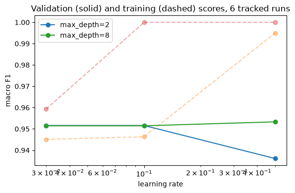

best = runs.loc[runs["val_f1_macro"].idxmax()]
print(f"winner on the VALIDATION split: run {best['run_id']} "
      f"(lr={best['learning_rate']}, depth={best['max_depth']}, "
      f"val F1={best['val_f1_macro']:.3f})")

winner on the VALIDATION split: run c7760640 (lr=0.5, depth=8, val F1=0.953)

Read the plot before moving on. The dashed training curves climb toward 1.0 as learning rate and depth grow, while the solid validation curves stay flat near 0.95 — the deep, aggressive models are memorizing the 5% label noise, and it buys them nothing on validation. With noisy labels, a training F1 of 1.000 is a warning, not an achievement. The only configuration that clearly loses is the most aggressive shallow one (learning rate 0.5, depth 2), which underfits the class structure while overreacting to noise.

Notice also how small the margins are: the top four configurations sit within a few thousandths of each other, and the “winner” leads by about 0.002. Hold that thought for the exercise.

Two rules we followed, both from the fair-evaluation thread of Chapters 3 and 4:

The winner is chosen on the validation split. The test split has not been touched. If we now reported the winner’s validation score as the headline result, it would be optimistically biased — we picked the maximum of six noisy numbers. The test split gets spent exactly once, at the end of the project.
Every number in the table traces to a run file with its parameters, code version, and timestamp. When a collaborator (or an agent, or reviewer 2) asks “how do you know which run was best?”, the answer is a file, not a memory.

What MLflow and Weights & Biases add¶

Our 30-line tracker records params, metrics, artifacts, and code version. That is also, exactly, the data model of the industrial tools — MLflow (open source, self-hosted or managed) and Weights & Biases (hosted service, free academic tier). What they add is engineering around the same four records:

A UI. Sortable run tables, parallel-coordinates plots, live-updating loss curves during training — our load_runs() and matplotlib, but instant and shareable.
Artifact stores. We logged artifact paths; they store the artifacts themselves (model weights, figures, datasets) with versioning and deduplication, so “the model from run 7f3a” is downloadable years later.
Collaboration. A team shares one tracking server; every group member’s runs land in the same searchable place, with access control. This is the difference that matters at lab scale.
Integrations. Autologging callbacks for scikit-learn, PyTorch, and friends record params and metrics without explicit log_run calls, plus hyperparameter-sweep orchestration.

The concepts are identical, and that is the point of having built the tracker yourself: when you adopt MLflow for your final project (encouraged), you know precisely what it is doing and what a runs/ directory of JSON would have given you for free. Use the real tools when you work with other people; never mistake them for the discipline itself.

Exercise: run-to-run variance¶

Your tracked study has one weakness: every run used seed=0. So “depth 8 beats depth 2 by 0.01” might be a fact, or might be luck of the initialization and subsampling.

Task. Using run_experiment, add tracked runs for the winning configuration with at least three different seeds. Load all runs, and quantify the run-to-run variance: mean, standard deviation, and range of val_f1_macro across seeds. Then answer: which differences in your six-run table are larger than the seed-to-seed spread — and therefore real?

Solution

# three more tracked runs, winning config, different seeds
for seed in [1, 2, 3]:
    run_experiment(learning_rate=best["learning_rate"],
                   max_depth=best["max_depth"], seed=seed)

runs = load_runs()
mask = ((runs["learning_rate"] == best["learning_rate"])
        & (runs["max_depth"] == best["max_depth"]))
spread = runs.loc[mask, "val_f1_macro"]
print(f"n={len(spread)}, mean={spread.mean():.4f}, "
      f"std={spread.std():.4f}, range={spread.max() - spread.min():.4f}")

Typical outcome on this data: a seed-to-seed standard deviation of a few thousandths in validation macro-F1. Now reread the pivot table with that ruler. The top four configurations differ by about the same few thousandths — including the “winner’s” 0.002 margin. Those differences are not findings; from single runs you cannot claim any of them is best, and the honest report is “indistinguishable at our run-to-run variance; we chose the shallowest, cheapest one.” The one gap that is many standard deviations wide is the drop to 0.936 at learning rate 0.5 with depth 2 — that configuration really is worse.

The general habit: any time you compare two configurations, know your seed-to-seed spread first. A difference smaller than the spread is not a finding. This is the cheapest ablation you will ever run, and the tracker made it three lines.