5.5 Data at Scale: Reading From Cloud Object Storage - Machine Learning in the Geosciences

Every dataset in this book so far fit in memory. This notebook works against one that does not: the MUR SST analysis — daily global sea-surface temperature at 0.01° (~1 km) resolution, 2002–2020, published as a Zarr store on the AWS Open Data registry (s3://mur-sst/zarr-v1, region us-west-2, anonymous access). Decoded, the store describes about 106 TiB of arrays. We will open it, subset it, and compute on it from a laptop, keeping one question front and center: how many bytes actually move?

This is the executable version of the “read in place” pattern from Section 5.4.

Data credit: JPL MUR MEaSUREs Project (2015), GHRSST Level 4 MUR Global Foundation Sea Surface Temperature Analysis v4.1, NASA PO.DAAC, NASA/JPL (2015); Chin, Vazquez-Cuervo & Armstrong (2017), Remote Sensing of Environment 200.

🖥️ Lecture slides — Session 27 (Fri Dec 4)

Reach the store — and fail fast if you cannot¶

One small object, .zmetadata, holds the store’s consolidated metadata: every array’s shape, dtype, chunking, and compression, in a single ~10 KiB read. We check it first with short timeouts, so a blocked network produces a clear error in seconds instead of a silent multi-minute hang.

import time

import numpy as np
import s3fs
import xarray as xr

STORE = "mur-sst/zarr-v1"
S3_OPTS = {
    "anon": True,  # public bucket, no credentials
    "config_kwargs": {"connect_timeout": 10, "read_timeout": 30, "retries": {"max_attempts": 2}},
}

fs = s3fs.S3FileSystem(**S3_OPTS)
try:
    meta = fs.info(f"{STORE}/.zmetadata")
except Exception as err:
    raise RuntimeError(
        f"Cannot reach s3://{STORE} (anonymous, region us-west-2). "
        "Check your connection. On restricted networks, outbound anonymous S3 is often "
        "blocked entirely -- see the admonition at the end of this notebook and the "
        "'Restricted environments' section of 5.4."
    ) from err


def fmt(nbytes):
    """Human-readable byte count."""
    for unit in ["B", "KiB", "MiB", "GiB", "TiB", "PiB"]:
        if nbytes < 1024:
            return f"{nbytes:,.1f} {unit}"
        nbytes /= 1024


print(f"store reachable; consolidated metadata: {fmt(meta['size'])} -- one GET describes everything below")

store reachable; consolidated metadata: 10.3 KiB -- one GET describes everything below

Open 106 TiB lazily¶

xr.open_dataset(..., engine="zarr", chunks={}) reads only that metadata object. chunks={} means “give me a dask array whose chunks match the chunks on disk” — no data values cross the network until we ask for them.

t0 = time.time()
ds = xr.open_dataset(
    f"s3://{STORE}",
    engine="zarr",
    chunks={},  # lazy: dask chunks = storage chunks
    backend_kwargs={"storage_options": S3_OPTS},
)
print(f"opened in {time.time() - t0:.1f} s: {fmt(ds.nbytes)} of arrays described, ~{fmt(meta['size'])} actually read")
ds

opened in 12.9 s: 106.3 TiB of arrays described, ~10.3 KiB actually read

Chunks: the unit of everything¶

A chunk is the store’s atomic unit of I/O and compression: every read fetches and decompresses whole chunks, never single values, so your access pattern pays in chunk-sized coins. Zarr v3 adds shards — many small chunks packed into one storage object so an object store is not drowned in millions of tiny files; this store predates them (Zarr v2 layout), so each chunk is one S3 object and the unit of network transfer.

analysed_sst is stored as int16 (a scale/offset pair reconstructs kelvins) in chunks of 5 days × 1799 lat × 3600 lon. Let us weigh one.

sst = ds["analysed_sst"]
storage_chunks = sst.encoding["chunks"]
chunk_of = dict(zip(sst.dims, storage_chunks))
print("shape:", sst.shape, "-> storage chunks:", storage_chunks)
print("stored dtype:", sst.encoding["dtype"], "| decoded dtype:", sst.dtype)

nchunks = tuple(int(np.ceil(s / c)) for s, c in zip(sst.shape, storage_chunks))
print("chunk grid:", nchunks, "=", f"{int(np.prod(nchunks)):,}", "chunk objects for this variable")

one = fs.info(f"{STORE}/analysed_sst/1200.7.1")  # one arbitrary chunk object
decoded_chunk = int(np.prod(storage_chunks)) * sst.dtype.itemsize
print(f"one chunk: {fmt(one['size'])} compressed on S3 -> {fmt(decoded_chunk)} decoded in RAM")
print(f"variable:  ~{fmt(one['size'] * np.prod(nchunks))} compressed (est. from that chunk) -> {fmt(sst.nbytes)} decoded")

# Rechunk on read: dask chunks must be multiples of the storage chunks, or every
# dask task re-reads partial storage chunks. This merges pairs of 5-day chunks:
sst10 = sst.chunk({"time": 10})  # equivalently: chunks={"time": 10, ...} in open_dataset
print("dask chunks after rechunk-on-read:", sst10.data.chunksize)

shape: (6443, 17999, 36000) -> storage chunks: (5, 1799, 3600)
stored dtype: int16 | decoded dtype: float64
chunk grid: (1289, 11, 10) = 141,790 chunk objects for this variable
one chunk: 20.0 MiB compressed on S3 -> 247.1 MiB decoded in RAM
variable:  ~2.7 TiB compressed (est. from that chunk) -> 30.4 TiB decoded

dask chunks after rechunk-on-read: (10, 1799, 3600)

Subset lazily, then compute¶

Ten days over the Pacific Northwest shelf: 46–49°N, 126–122°W, June 2019. Slicing a lazy array edits the task graph — it still moves zero bytes.

TIME = slice("2019-06-01", "2019-06-10")
LAT, LON = slice(46, 49), slice(-126, -122)

sub = sst.sel(time=TIME, lat=LAT, lon=LON)
print(f"subset {sub.shape}: {fmt(sub.data.nbytes)} across {sub.data.npartitions} chunks -- 0 bytes moved so far")

subset (10, 301, 401): 9.2 MiB across 3 chunks -- 0 bytes moved so far

.compute() is where the network bill arrives. Two different byte counts matter, and we measure both:

bytes in RAM — dask’s nbytes on the computed result: what your answer costs in memory;
bytes moved — the network transfers whole compressed chunk objects, so we list exactly which chunk objects the subset touches and sum their sizes on S3.

t0 = time.time()
box = sub.compute()
elapsed = time.time() - t0

# Which chunk objects did that read touch? Convert the label slices to integer
# index ranges, divide by the chunk size along each dimension, and list the keys.
ranges = {}
for dim, sel in {"time": TIME, "lat": LAT, "lon": LON}.items():
    start, stop = sst.get_index(dim).slice_locs(sel.start, sel.stop)
    ranges[dim] = range(start // chunk_of[dim], (stop - 1) // chunk_of[dim] + 1)
keys = [
    f"{STORE}/analysed_sst/{t}.{y}.{x}"
    for t in ranges["time"] for y in ranges["lat"] for x in ranges["lon"]
]
moved = sum(fs.info(k)["size"] for k in keys)

print(f"chunk objects fetched : {len(keys)} (= {sub.data.npartitions} graph partitions)")
print(f"bytes moved           : {fmt(moved)} compressed, in {elapsed:.1f} s")
print(f"bytes in RAM (result) : {fmt(box.nbytes)}")
print(f"bytes stored (decoded): {fmt(sst.nbytes)}")
print(f"moved : stored        = 1 : {sst.nbytes / moved:,.0f}")
print(f"mean SST in the box   : {float(box.mean()):.2f} K")

chunk objects fetched : 3 (= 3 graph partitions)
bytes moved           : 60.6 MiB compressed, in 20.4 s
bytes in RAM (result) : 9.2 MiB
bytes stored (decoded): 30.4 TiB
moved : stored        = 1 : 525,483
mean SST in the box   : 285.94 K

That ratio is the entire argument for cloud-optimized formats. The store holds 30.4 TiB (decoded) of analysed_sst; answering our question moved 60.6 MiB — one part in ~525,000 — because chunking makes partial reads cheap and laziness means we only ever asked for the chunks our slice touches. The 60.6 MiB is also ~6× larger than the 9.2 MiB that landed in RAM: chunk granularity is the tax you pay for object storage, and why chunk shape should roughly match your access pattern.

The moment in-memory dies¶

Do the arithmetic before you ever call .compute() on something big. One global timestep of analysed_sst decodes to 17,999 × 36,000 × 8 bytes ≈ 4.8 GiB. Three days exhausts a 16 GiB laptop. The full variable is 30.4 TiB — about two thousand laptops of RAM — and sst.values (or .compute() on the unsubset array) would cheerfully try to materialize it. We are not going to run that, and neither should you: the fix is never a bigger .compute(), it is an algorithm that holds only a few chunks at a time.

Streaming: the aggregation that succeeds¶

A monthly mean over the same box needs 30 global days — ~145 GiB decoded if you loaded whole timesteps, but still only 7 chunk objects for our slice. mean("time") on the lazy array builds a graph of per-chunk partial means that dask combines: each worker fetches one 20 MiB chunk object, decompresses it (62 MiB of int16, 247 MiB once decoded to float64), takes its partial mean over the slice, and drops it. Peak memory stays at a handful of chunks no matter how long the time axis gets.

june = sst.sel(time=slice("2019-06-01", "2019-06-30"), lat=LAT, lon=LON)
june_mean = june.mean("time")  # lazy: per-chunk partial means, combined at the end

print(f"graph input : {fmt(june.data.nbytes)} across {june.data.npartitions} chunks")
print(f"graph output: {fmt(june_mean.data.nbytes)}")

t0 = time.time()
june_map = june_mean.compute()
print(f"streamed in {time.time() - t0:.1f} s; peak memory ~ a few chunks, not {fmt(sst.nbytes)}")

graph input : 27.6 MiB across 7 chunks
graph output: 943.0 KiB

streamed in 40.8 s; peak memory ~ a few chunks, not 30.4 TiB

import matplotlib.pyplot as plt

june_map.plot(figsize=(7, 4), cmap="viridis", cbar_kwargs={"label": "mean SST (K)"})
plt.title("MUR SST, June 2019 mean -- Pacific Northwest coast")
plt.tight_layout()
plt.show()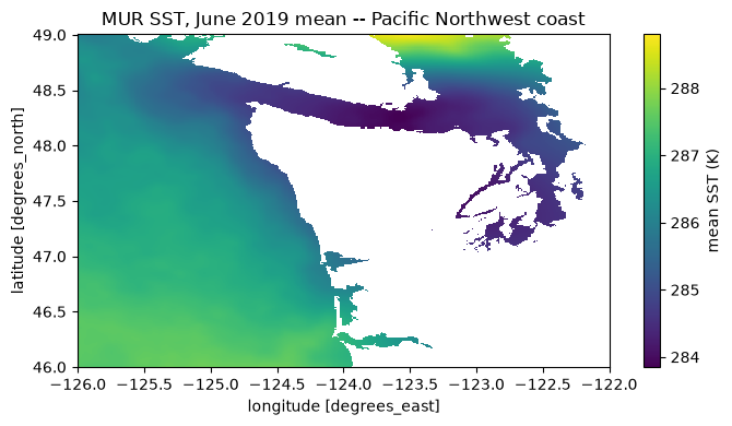

Anonymous S3 reads fail on restricted networks

On many institutional networks — national labs, agency enclaves, some campus HPC compute nodes — outbound anonymous S3 is blocked. The symptom is rarely a clean error: the open hangs for the length of the timeout, then raises ConnectTimeoutError/EndpointConnectionError, or a proxy answers with a misleading 403. (This notebook’s first cell uses 10-second timeouts and a plain-language error precisely so the failure is fast and legible.) The fallback is not to fight the firewall: use an institutional mirror of the archive if one exists, or pre-stage a subset — run the subsetting cells on a connected machine, box.to_netcdf(...) the result (9.2 MiB, not 30.4 TiB), move it through your approved transfer gateway, and pin its hash with pooch (Section 1.6). The environment side of the same problem is covered in 5.4, “Restricted environments”.

Laptop → HPC → cloud: the decision in numbers¶

This notebook answered questions about a 30.4 TiB variable by moving ~200 MiB total — comfortably a laptop job, because the chunks we touched fit our bandwidth and RAM. That is the general rule:

Chunks you touch ≪ your RAM and patience → laptop, exactly as here. Lazy open, subset, stream.
Chunks you touch ≈ the whole store (a global, full-record climatology; ML training over every chunk) → move the compute to the data, not the data to the compute: an instance in us-west-2 reads this bucket at multi-GB/s with no egress fee, and an HPC cluster works when the data (or a mirror) is already on its filesystem.
Either way, the query travels to the data and only answers travel back — the “read in place” pattern of Section 5.4, which also covers the compute ladder itself: departmental cluster, NSF ACCESS, commercial cloud, and the cost discipline that keeps the last one survivable.

References¶

NASA/JPL. (2015). GHRSST Level 4 MUR Global Foundation Sea Surface Temperature Analysis (v4.1). NASA Physical Oceanography Distributed Active Archive Center. 10.5067/GHGMR-4FJ04