Tutorial 1: Background and data preparation#
Outline#
Imports
Brief discussion of xarray, intake, and zarr
Brief discussion of ERA5, SRTM, and CMIP6 + downscaling
Introduction to
torchdata.datapipesWalk through of data processing steps
Subsetting to a region
Scaling/normalizing the data
Conversion between spatio-temporal dataset and ML-ready samples
Data splitting for train-valid-test splits
Demonstration of the total pipeline and export to library code for next steps
Package installation and imports#
Before we can get to the fun stuff we must start by setting up an environment with some basic packages as well as some specialized packages. This tutorial assumes that you are running on the Microsoft Planetary Computer, which comes with a preconfigured environment with many packages for Earth science and machine learning. If you are running somewhere else you may need to install from the conda environment provided at the base of the tutorial. That said, here we will install all the stuff we need.
A quick rundown of what this all is:
zarr: The data format that we will be usingtorchdata: Additional data handling routines for pytorchzen3geo: Additional data handling routines that connecttorchdataandxbatcherdask: Allows for parallel processingintake: A library for using catalogues to manage datasetsxarray: The data model we will use for labeled n-dimensional arrays, can interoperate well withzarrandintakefsspec,aiohttp: Allows for opening zarr files over networkregionmask: Makes it easy to subset geographic regions from datasetscmip6-downscaling: Provides tools for accessing the CarbonPlan CMIP6 downscaled dataxbatcher: Tools for using machine learning onxarraydatasets
!pip install -q zarr torchdata zen3geo dask[distributed] intake xarray fsspec aiohttp regionmask --upgrade
!pip install -q git+https://github.com/carbonplan/cmip6-downscaling.git@1.0
!pip install -q git+https://github.com/xarray-contrib/xbatcher.git@463546e7739e68b10f1ae456fb910a1628de1e5c
import os
import torch
import intake
import regionmask
import xbatcher
import xarray as xr
import numpy as np
import matplotlib.pyplot as plt
import warnings
import zen3geo

from tqdm.autonotebook import tqdm
from functools import partial
from dask.distributed import Client, LocalCluster
from torchdata.datapipes.iter import IterDataPipe
from torch.utils.data import DataLoader

warnings.filterwarnings('ignore')
DEVICE = torch.device("cuda:0" if torch.cuda.is_available() else "cpu")
DTYPE = torch.float32
/tmp/ipykernel_4786/154572687.py:12: TqdmExperimentalWarning: Using `tqdm.autonotebook.tqdm` in notebook mode. Use `tqdm.tqdm` instead to force console mode (e.g. in jupyter console)
  from tqdm.autonotebook import tqdm
import matplotlib as mpl
import matplotlib.pyplot as plt
mpl.rcParams['figure.dpi'] = 300
Opening the data#
Actually getting data into order and merged together is usually one of the hardest parts of the machine learning pipeline for new tasks. In common fashion, we have some work ahead of ourselves. Luckily, all of the data is readily available via publicly accessible cloud datasets that can be opened over the network, which means you don’t actually have to download anything directly!
We can see the overall data by using the intake catalog provided by CarbonPlan:
era5_daily_cat = intake.open_esm_datastore(
    'https://cpdataeuwest.blob.core.windows.net/cp-cmip/training/ERA5-daily-azure.json'
)
era5_daily_cat
ERA5-azure catalog with 546 dataset(s) from 546 asset(s):
| unique | |
|---|---|
| year | 42 |
| month | 1 |
| standard_name | 13 |
| product_type | 2 |
| short_name | 13 |
| cf_variable_name | 13 |
| aggregation_method | 4 |
| units | 5 |
| zstore | 42 |
| timescale | 1 |
| time | 42 |
| derived_standard_name | 0 |
From this we can see a number of things inside of the catalog, most salient that there are 42 years of data with 13 variables and 4 aggregation methods. Let’s dig in deeper by searching for which unique variables exist in the data:
era5_daily_cat.unique()['cf_variable_name']
['psl',
 'tas',
 'tasmax',
 'tasmin',
 'tdps',
 'ua100m',
 'uas',
 'rsds',
 'va100m',
 'vas',
 'pr',
 'tos',
 'ps']
Now this might not be quite so helpful if you are new to ERA5 data, so instead let’s look at the standard_name which is a bit more intuitive. From this we can better understand the actual data inside of this catalog. Looking through this, we will make the call to use variables:
tasmax:'air_temperature_at_2_metres_1hour_Maximum'tasmin:'air_temperature_at_2_metres_1hour_Minimum'pr:'precipitation_amount_1hour_Accumulation'
The reason for these choices is because this is what is included in the downscaled CMIP6 data that we will use in the last portion of this tutorial.
era5_daily_cat.unique()['standard_name']
['air_pressure_at_mean_sea_level',
 'air_temperature_at_2_metres',
 'air_temperature_at_2_metres_1hour_Maximum',
 'air_temperature_at_2_metres_1hour_Minimum',
 'dew_point_temperature_at_2_metres',
 'eastward_wind_at_100_metres',
 'eastward_wind_at_10_metres',
 'integral_wrt_time_of_surface_direct_downwelling_shortwave_flux_in_air_1hour_Accumulation',
 'northward_wind_at_100_metres',
 'northward_wind_at_10_metres',
 'precipitation_amount_1hour_Accumulation',
 'sea_surface_temperature',
 'surface_air_pressure']
From this we can search out the data that has these variables. Then, we use the df accessor to get the underlying dataframe which let’s us acces the zstore attribute, which is a URL to a zarr file that we can open. But, searching this returns a sequence of zarr stores, so before we attempt to open them we will convert them to a list and then sort them. For the example we will just find the files that have the tasmax variable, and coincidentally also include the tasmin and pr variables which are everything we will use to develop our models! You should verify this yourself by searching for the other variable names and seeing that the underlying stores are the same.
met_files = sorted(list(era5_daily_cat.search(cf_variable_name='tasmin').df['zstore']))
met_files
['https://cpdataeuwest.blob.core.windows.net/cp-cmip/training/ERA5_daily/1979',
 'https://cpdataeuwest.blob.core.windows.net/cp-cmip/training/ERA5_daily/1980',
 'https://cpdataeuwest.blob.core.windows.net/cp-cmip/training/ERA5_daily/1981',
 'https://cpdataeuwest.blob.core.windows.net/cp-cmip/training/ERA5_daily/1982',
 'https://cpdataeuwest.blob.core.windows.net/cp-cmip/training/ERA5_daily/1983',
 'https://cpdataeuwest.blob.core.windows.net/cp-cmip/training/ERA5_daily/1984',
 'https://cpdataeuwest.blob.core.windows.net/cp-cmip/training/ERA5_daily/1985',
 'https://cpdataeuwest.blob.core.windows.net/cp-cmip/training/ERA5_daily/1986',
 'https://cpdataeuwest.blob.core.windows.net/cp-cmip/training/ERA5_daily/1987',
 'https://cpdataeuwest.blob.core.windows.net/cp-cmip/training/ERA5_daily/1988',
 'https://cpdataeuwest.blob.core.windows.net/cp-cmip/training/ERA5_daily/1989',
 'https://cpdataeuwest.blob.core.windows.net/cp-cmip/training/ERA5_daily/1990',
 'https://cpdataeuwest.blob.core.windows.net/cp-cmip/training/ERA5_daily/1991',
 'https://cpdataeuwest.blob.core.windows.net/cp-cmip/training/ERA5_daily/1992',
 'https://cpdataeuwest.blob.core.windows.net/cp-cmip/training/ERA5_daily/1993',
 'https://cpdataeuwest.blob.core.windows.net/cp-cmip/training/ERA5_daily/1994',
 'https://cpdataeuwest.blob.core.windows.net/cp-cmip/training/ERA5_daily/1995',
 'https://cpdataeuwest.blob.core.windows.net/cp-cmip/training/ERA5_daily/1996',
 'https://cpdataeuwest.blob.core.windows.net/cp-cmip/training/ERA5_daily/1997',
 'https://cpdataeuwest.blob.core.windows.net/cp-cmip/training/ERA5_daily/1998',
 'https://cpdataeuwest.blob.core.windows.net/cp-cmip/training/ERA5_daily/1999',
 'https://cpdataeuwest.blob.core.windows.net/cp-cmip/training/ERA5_daily/2000',
 'https://cpdataeuwest.blob.core.windows.net/cp-cmip/training/ERA5_daily/2001',
 'https://cpdataeuwest.blob.core.windows.net/cp-cmip/training/ERA5_daily/2002',
 'https://cpdataeuwest.blob.core.windows.net/cp-cmip/training/ERA5_daily/2003',
 'https://cpdataeuwest.blob.core.windows.net/cp-cmip/training/ERA5_daily/2004',
 'https://cpdataeuwest.blob.core.windows.net/cp-cmip/training/ERA5_daily/2005',
 'https://cpdataeuwest.blob.core.windows.net/cp-cmip/training/ERA5_daily/2006',
 'https://cpdataeuwest.blob.core.windows.net/cp-cmip/training/ERA5_daily/2007',
 'https://cpdataeuwest.blob.core.windows.net/cp-cmip/training/ERA5_daily/2008',
 'https://cpdataeuwest.blob.core.windows.net/cp-cmip/training/ERA5_daily/2009',
 'https://cpdataeuwest.blob.core.windows.net/cp-cmip/training/ERA5_daily/2010',
 'https://cpdataeuwest.blob.core.windows.net/cp-cmip/training/ERA5_daily/2011',
 'https://cpdataeuwest.blob.core.windows.net/cp-cmip/training/ERA5_daily/2012',
 'https://cpdataeuwest.blob.core.windows.net/cp-cmip/training/ERA5_daily/2013',
 'https://cpdataeuwest.blob.core.windows.net/cp-cmip/training/ERA5_daily/2014',
 'https://cpdataeuwest.blob.core.windows.net/cp-cmip/training/ERA5_daily/2015',
 'https://cpdataeuwest.blob.core.windows.net/cp-cmip/training/ERA5_daily/2016',
 'https://cpdataeuwest.blob.core.windows.net/cp-cmip/training/ERA5_daily/2017',
 'https://cpdataeuwest.blob.core.windows.net/cp-cmip/training/ERA5_daily/2018',
 'https://cpdataeuwest.blob.core.windows.net/cp-cmip/training/ERA5_daily/2019',
 'https://cpdataeuwest.blob.core.windows.net/cp-cmip/training/ERA5_daily/2020']
Given this list of zarr stores we can then simply open them up with xarray via the open_mfdataset function (which stands for “open multi file dataset). Upon inspection you can see that this has the entire dataset including many more variables than we need. It is also a global dataset containing daily values from 1979 through 2020.
met_ds = xr.open_mfdataset(met_files, engine='zarr')
met_ds
<xarray.Dataset>
Dimensions:  (lat: 721, lon: 1440, time: 15341)
Coordinates:
  * lat      (lat) float32 90.0 89.75 89.5 89.25 ... -89.25 -89.5 -89.75 -90.0
  * lon      (lon) float32 0.0 0.25 0.5 0.75 1.0 ... 359.0 359.2 359.5 359.8
  * time     (time) datetime64[ns] 1979-01-01 1979-01-02 ... 2020-12-31
Data variables: (12/13)
    pr       (time, lat, lon) float64 dask.array<chunksize=(365, 150, 150), meta=np.ndarray>
    ps       (time, lat, lon) float32 dask.array<chunksize=(365, 150, 150), meta=np.ndarray>
    psl      (time, lat, lon) float32 dask.array<chunksize=(365, 150, 150), meta=np.ndarray>
    rsds     (time, lat, lon) float64 dask.array<chunksize=(365, 150, 150), meta=np.ndarray>
    tas      (time, lat, lon) float32 dask.array<chunksize=(365, 150, 150), meta=np.ndarray>
    tasmax   (time, lat, lon) float32 dask.array<chunksize=(365, 150, 150), meta=np.ndarray>
    ...       ...
    tdps     (time, lat, lon) float32 dask.array<chunksize=(365, 150, 150), meta=np.ndarray>
    tos      (time, lat, lon) float32 dask.array<chunksize=(365, 150, 150), meta=np.ndarray>
    ua100m   (time, lat, lon) float32 dask.array<chunksize=(365, 150, 150), meta=np.ndarray>
    uas      (time, lat, lon) float32 dask.array<chunksize=(365, 150, 150), meta=np.ndarray>
    va100m   (time, lat, lon) float32 dask.array<chunksize=(365, 150, 150), meta=np.ndarray>
    vas      (time, lat, lon) float32 dask.array<chunksize=(365, 150, 150), meta=np.ndarray>
Attributes:
    institution:  ECMWF
    source:       Reanalysis
title: ERA5 forecastsIf you look at all of the variables that exist in the met_ds dataset from our previous query you’ll see they provide daily minimum temperature, daily maximum temperature, and precipitation rates. Without getting too into things, this is all we need as far as external forcings/meteorological data because this is generally the basics that are provided by climate projections. We’ll see this bear out later when we actually get to using our trained model to make climate projections.
You will also notice if you look through the data in met_ds that there is no snow, which we definitely will need. The snow product we will use is in a different dataset, and can be opened up with the following code:
years = np.arange(1985, 2015)
swe_files = [f'https://esiptutorial.blob.core.windows.net/eraswe/era5_raw_swe/era5_raw_swe_{year}.zarr'
             for year in years]
swe_ds = xr.open_mfdataset(swe_files, engine='zarr')
daily_swe = swe_ds.resample(time='1D').mean().rename({'latitude': 'lat', 'longitude': 'lon'})
daily_swe
<xarray.Dataset>
Dimensions:  (time: 10957, lat: 721, lon: 1440)
Coordinates:
  * lat      (lat) float32 90.0 89.75 89.5 89.25 ... -89.25 -89.5 -89.75 -90.0
  * lon      (lon) float32 0.0 0.25 0.5 0.75 1.0 ... 359.0 359.2 359.5 359.8
  * time     (time) datetime64[ns] 1985-01-01 1985-01-02 ... 2014-12-31
Data variables:
    sd       (time, lat, lon) float32 dask.array<chunksize=(46, 91, 180), meta=np.ndarray>
Attributes:
    Conventions:  CF-1.6
history: 2022-07-22 01:22:35 GMT by grib_to_netcdf-2.25.1: /opt/ecmw...We did a daily resampling on this because the data actually provides a daytime value and a night time value for the snow, but we’ll assume that they don’t change too much for our purposes here and just take the mean of them together via the resample method. We also have to rename the coordinate names so that we can merge them together with the meteorologic data.
Finally, just having meteorologic data and snow data is good, but possibly not enough for the model. We’ll also be including some static spatial attributes like the elevation, aspect, and slope for each location in the data. These were derived from the SRTM satellite data. There is also a mask that we developed to select where to include training data from. This mask essentially is looking for areas where there is enough snow to be informative for the model.
mask = xr.open_dataset(
    'https://esiptutorial.blob.core.windows.net/eraswe/mask_10k_household.zarr',
    engine='zarr'
)
mask = mask.rename({'latitude': 'lat', 'longitude': 'lon', 'sd': 'mask'})
terrain = xr.open_dataset(
    'https://esiptutorial.blob.core.windows.net/eraswe/processed_slope_aspect_elevation.zarr',
    engine='zarr'
)
terrain['mask'] = mask['mask']
terrain['mask'] = np.logical_and(~np.isnan(terrain['elevation']), terrain['mask']>0 ).astype(int)
terrain
<xarray.Dataset>
Dimensions:        (lat: 721, lon: 1440)
Coordinates:
  * lat            (lat) float32 90.0 89.75 89.5 89.25 ... -89.5 -89.75 -90.0
  * lon            (lon) float32 0.0 0.25 0.5 0.75 ... 359.0 359.2 359.5 359.8
Data variables:
    aspect_cosine  (lat, lon) float64 ...
    aspect_sine    (lat, lon) float64 ...
    elevation      (lat, lon) float64 0.0 0.0 0.0 0.0 0.0 ... 0.0 0.0 0.0 0.0
    slope          (lat, lon) float64 ...
    mask           (lat, lon) int64 0 0 0 0 0 0 0 0 0 0 ... 0 0 0 0 0 0 0 0 0 0
Attributes:
regrid_method: bilinearPutting it all together#
With all of the data opened up, we can simply merge it together into a single dataset which will make working with it a bit simpler.
xr.merge([met_ds, daily_swe, terrain])
<xarray.Dataset>
Dimensions:        (lat: 721, lon: 1440, time: 15341)
Coordinates:
  * lat            (lat) float32 90.0 89.75 89.5 89.25 ... -89.5 -89.75 -90.0
  * lon            (lon) float32 0.0 0.25 0.5 0.75 ... 359.0 359.2 359.5 359.8
  * time           (time) datetime64[ns] 1979-01-01 1979-01-02 ... 2020-12-31
Data variables: (12/19)
    pr             (time, lat, lon) float64 dask.array<chunksize=(365, 150, 150), meta=np.ndarray>
    ps             (time, lat, lon) float32 dask.array<chunksize=(365, 150, 150), meta=np.ndarray>
    psl            (time, lat, lon) float32 dask.array<chunksize=(365, 150, 150), meta=np.ndarray>
    rsds           (time, lat, lon) float64 dask.array<chunksize=(365, 150, 150), meta=np.ndarray>
    tas            (time, lat, lon) float32 dask.array<chunksize=(365, 150, 150), meta=np.ndarray>
    tasmax         (time, lat, lon) float32 dask.array<chunksize=(365, 150, 150), meta=np.ndarray>
    ...             ...
    sd             (time, lat, lon) float32 dask.array<chunksize=(2238, 91, 180), meta=np.ndarray>
    aspect_cosine  (lat, lon) float64 ...
    aspect_sine    (lat, lon) float64 ...
    elevation      (lat, lon) float64 0.0 0.0 0.0 0.0 0.0 ... 0.0 0.0 0.0 0.0
    slope          (lat, lon) float64 ...
    mask           (lat, lon) int64 0 0 0 0 0 0 0 0 0 0 ... 0 0 0 0 0 0 0 0 0 0
Attributes:
    institution:  ECMWF
    source:       Reanalysis
title: ERA5 forecastsAnd to go one step further, let’s just wrap all of that code into one nice, handy function that we can put into a code module and use from here on out without worrying about the details of how we did the reorganizing and merging. The last little thing we’ll throw in there is taking a cubed root for the SWE and precip variables, which will help us to better normalize the data for training time.
def merge_data():
    # SWE Data
    years = np.arange(1985, 2015)
    swe_files = [f'https://esiptutorial.blob.core.windows.net/eraswe/era5_raw_swe/era5_raw_swe_{year}.zarr'
                 for year in years]
    swe_ds = xr.open_mfdataset(swe_files, engine='zarr')
    daily_swe = swe_ds.resample(time='1D').mean().rename({'latitude': 'lat', 'longitude': 'lon'})
    daily_swe = daily_swe.rename({'sd': 'swe'})

    # Meteorological forcings
    era5_daily_cat = intake.open_esm_datastore(
        'https://cpdataeuwest.blob.core.windows.net/cp-cmip/training/ERA5-daily-azure.json'
    )
    met_files = sorted(list(era5_daily_cat.search(cf_variable_name='tasmax').df['zstore']))
    met_ds = xr.open_mfdataset(met_files,  engine='zarr')
    met_ds = met_ds.sel(time=slice(daily_swe['time'].min(), daily_swe['time'].max()))

    # Terrain data
    mask = xr.open_dataset(
        'https://esiptutorial.blob.core.windows.net/eraswe/mask_10k_household.zarr',
    engine='zarr'
    )
    mask = mask.rename({'latitude': 'lat', 'longitude': 'lon', 'sd': 'mask'})
    terrain = xr.open_dataset(
        'https://esiptutorial.blob.core.windows.net/eraswe/processed_slope_aspect_elevation.zarr',
        engine='zarr'
    )
    terrain['mask'] = mask['mask']
    terrain['mask'] = np.logical_and(~np.isnan(terrain['elevation']), terrain['mask']>0 ).astype(int)
    ds = xr.merge([met_ds, daily_swe, terrain])
    ds['cbrt_swe'] = np.power(ds['swe'], 1/3)
    ds['cbrt_pr'] = np.power(ds['pr'], 1/3)
    return ds

ds = merge_data()
ds
<xarray.Dataset>
Dimensions:        (lat: 721, lon: 1440, time: 10957)
Coordinates:
  * lat            (lat) float32 90.0 89.75 89.5 89.25 ... -89.5 -89.75 -90.0
  * lon            (lon) float32 0.0 0.25 0.5 0.75 ... 359.0 359.2 359.5 359.8
  * time           (time) datetime64[ns] 1985-01-01 1985-01-02 ... 2014-12-31
Data variables: (12/21)
    pr             (time, lat, lon) float64 dask.array<chunksize=(365, 150, 150), meta=np.ndarray>
    ps             (time, lat, lon) float32 dask.array<chunksize=(365, 150, 150), meta=np.ndarray>
    psl            (time, lat, lon) float32 dask.array<chunksize=(365, 150, 150), meta=np.ndarray>
    rsds           (time, lat, lon) float64 dask.array<chunksize=(365, 150, 150), meta=np.ndarray>
    tas            (time, lat, lon) float32 dask.array<chunksize=(365, 150, 150), meta=np.ndarray>
    tasmax         (time, lat, lon) float32 dask.array<chunksize=(365, 150, 150), meta=np.ndarray>
    ...             ...
    aspect_sine    (lat, lon) float64 ...
    elevation      (lat, lon) float64 0.0 0.0 0.0 0.0 0.0 ... 0.0 0.0 0.0 0.0
    slope          (lat, lon) float64 ...
    mask           (lat, lon) int64 0 0 0 0 0 0 0 0 0 0 ... 0 0 0 0 0 0 0 0 0 0
    cbrt_swe       (time, lat, lon) float32 dask.array<chunksize=(46, 91, 180), meta=np.ndarray>
    cbrt_pr        (time, lat, lon) float64 dask.array<chunksize=(365, 150, 150), meta=np.ndarray>
Attributes:
    institution:  ECMWF
    source:       Reanalysis
title: ERA5 forecastsIntroduction to torchdata.datapipes#
Before we dive into how we can process this data, let’s take a quick side diversion into the torchdata package which
is designed to help with the creation and management of PyTorch datasets. Particularly, we’ll use the datapipesthat provides a set of tools for efficiently loading and transforming data. The key benefit of datapipe is its ability to process data in a streaming fashion, which can significantly reduce the memory usage and processing time of the data loading pipeline.
class RandomNumbersPipe(IterDataPipe):

    def __init__(self, sample_shape, number_samples):
        super().__init__()
        self.sample_shape = sample_shape
        self.number_samples = number_samples

    def __iter__(self):
        for _ in range(self.number_samples):
            yield torch.randn(self.sample_shape)
randoms = RandomNumbersPipe(sample_shape=(5,2,), number_samples=3)
for sample in randoms:
    print(f'Shape: {sample.shape}, Mean: {torch.mean(sample)}')
Shape: torch.Size([5, 2]), Mean: 0.10140786319971085
Shape: torch.Size([5, 2]), Mean: 0.11181142181158066
Shape: torch.Size([5, 2]), Mean: 0.016363954171538353
The datapipe approach makes it easy to apply transformation functions that can be used to preprocess data as it is loaded. These functions can be chained together to form a pipeline, allowing for complex data transformations to be performed with ease. We’ll make use of this to go from the raw, gridded datasets to something that is usable by our model that we’ll define in the next tutorial notebook. For now, let’s suppose that we simply want to transpose the numbers that come out of the RandomNumbersPipe that we used earlier. This is easy enough to write as a simple function, which we call transpose below:
def transpose(x):
    return x.T
With this in hand, we can simply call the map method on the randoms pipe, which produces a new datapipe that can be iterated over. This can easily be seen below:
randoms = RandomNumbersPipe(sample_shape=(5,2,), number_samples=3)
transposed = randoms.map(transpose)

for sample in transposed:
    print(f'Shape: {sample.shape}, Mean: {torch.mean(sample)}')
Shape: torch.Size([2, 5]), Mean: -0.5375681519508362
Shape: torch.Size([2, 5]), Mean: 0.1900019645690918
Shape: torch.Size([2, 5]), Mean: -0.3826327919960022
The extract-transform-load (ETL) pipeline#
Now that we know how to access the raw data and have a basic strategy for manipulating said data into something that can ostensibly be used for training a recurrent neural network (RNN). Our basic starting point will be to subset the global data down to a region of interest. As mentioned in other parts of the tutorial, we take this approach simply to reduce the computational workload and make it easy to run this example in an end-to-end fashion in a timely manner. To do this we will first implement a new RegionalSubsetterPipe class which takes the full dataset and a list of regions from the regions defined in Giorgi and Francisco (2020) and dynamically select only one region at a time. In addition to the benefit of making it easy to run this tutorial on limited time/compute, this actually has another practical benefit for running global analyses - which is that most of the gridcells in the global domain actually are not located in areas that we have flagged for snow modeling via the mask variable. This regional subsetting means we will have far fewer samples to filter out at training time, which will lower not only the training time but the amount of data that is ultimately transferred over the wire and processed. This type of approach, where we are using
publicly provided, large, “analysis-ready” datasets is very useful for reproducibility, accessiblility, proof-of-concept research, and learning materials. For larger projects and mature research programs, it usually will be better to actually process the data similarly to what we do here, but save the intermediate samples out to disk/cloud storage directly and avoid the computation associated with the sampling process.
Anyhow, we can define the RegionalSubsetterPipe in a relatively straightforward manner, by taking in the full dataset, a sequence of the regions that are to be processed, and optionally a flag for whether to load an entire region into memory up front. The mechancs for actually selecting the region from the raw dataset is slightly involved, so we will walk through that piece in a bit more detail. First, here’s the full class:
class RegionalSubsetterPipe(IterDataPipe):

    def __init__(self, ds, selected_regions=None, preload=False):
        super().__init__()
        self.ds = ds
        self.selected_regions = self.to_sequence(selected_regions)
        self.preload = preload

    def to_sequence(self, seq):
        if isinstance(seq, str):
            return (seq, )
        return seq

    def __iter__(self):
        if not self.selected_regions:
            yield self.ds
        else:
            for region in self.selected_regions:
                self.selected_ds = select_region(self.ds, region)
                if self.preload:
                    self.selected_ds = self.selected_ds.load()
                yield self.selected_ds
If you study the RegionalSubsetterPipe code closely, you’ll note that it calls the select_region function inside of the __iter__ method. This hasn’t been defined or imported yet, so before we can actually use this we’ll have to figure out a way to select a single region from a given xarray dataset. Luckily, most of the functionality for this has already been developed in the regionmask package which we installed in the first cell.
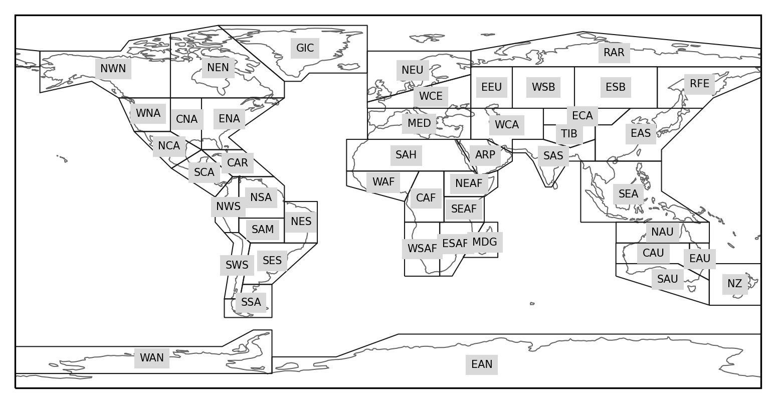
Given that, we can define the function, which takes a dataset and the string name of a particular region from the regionmask.defined_regions.ar6.land attribute. You can look at that on your own if you’re interested in what it contains, but for now we can just make a plot of all of the regions and their abbreviations so that you can easily select regions of interest. Note, in the given tutorial we will be assuming you are using the WNA region, but the code should be relatively straightforward enough to modify for other regions.
regionmask.defined_regions.ar6.land.plot(
    label='abbrev',
    text_kws={'fontsize': 5},
    line_kws={'linewidth':0.5}
)
<GeoAxesSubplot:>
Getting back to the task at hand, we just need a function which takes a dataset and a region as a string and then subsets it to the given region. This can be done with regionmask’s built in functionality for masking. Given this we just have to find the regions which match the given mask, and then subset them. This is handled below, but we recommend you play with the steps individually if you want to learn how they work in-depth.
def select_region(ds, region):
    # Get all regions & create mask from lat/lons
    regions = regionmask.defined_regions.ar6.land
    region_id_mask = regions.mask(ds['lon'], ds['lat'])
    # Get unique listing of region names & abbreviations
    reg = np.unique(region_id_mask.values)
    reg = reg[~np.isnan(reg)]
    region_abbrevs = np.array(regions[reg].abbrevs)
    region_names = np.array(regions[reg].names)
    # Create a mask that only contains the region of interest
    selection_mask = 0.0 * region_id_mask.copy()
    region_idx = np.argwhere(region_abbrevs == region)[0][0]
    region_mask = (region_id_mask == reg[region_idx]).astype(int)
    return ds.where(region_mask, drop=True)
As mentioned earlier, one of the benefits of working in the data-pipe framework is we can iteratively develop and test each component of the ETL pipeline in a flexible and modular way that fits really nicely into the Jupyter workflow. To see this in action, let’s actually instantiate and test if this behaves as expected!
r = RegionalSubsetterPipe(ds, 'WNA')
for subset in r:
    print(subset.dims)
    print(subset.coords)
Frozen({'time': 10957, 'lat': 65, 'lon': 100})
Coordinates:
  * lat      (lat) float32 50.0 49.75 49.5 49.25 49.0 ... 34.75 34.5 34.25 34.0
  * lon      (lon) float32 230.2 230.5 230.8 231.0 ... 254.2 254.5 254.8 255.0
  * time     (time) datetime64[ns] 1985-01-01 1985-01-02 ... 2014-12-31
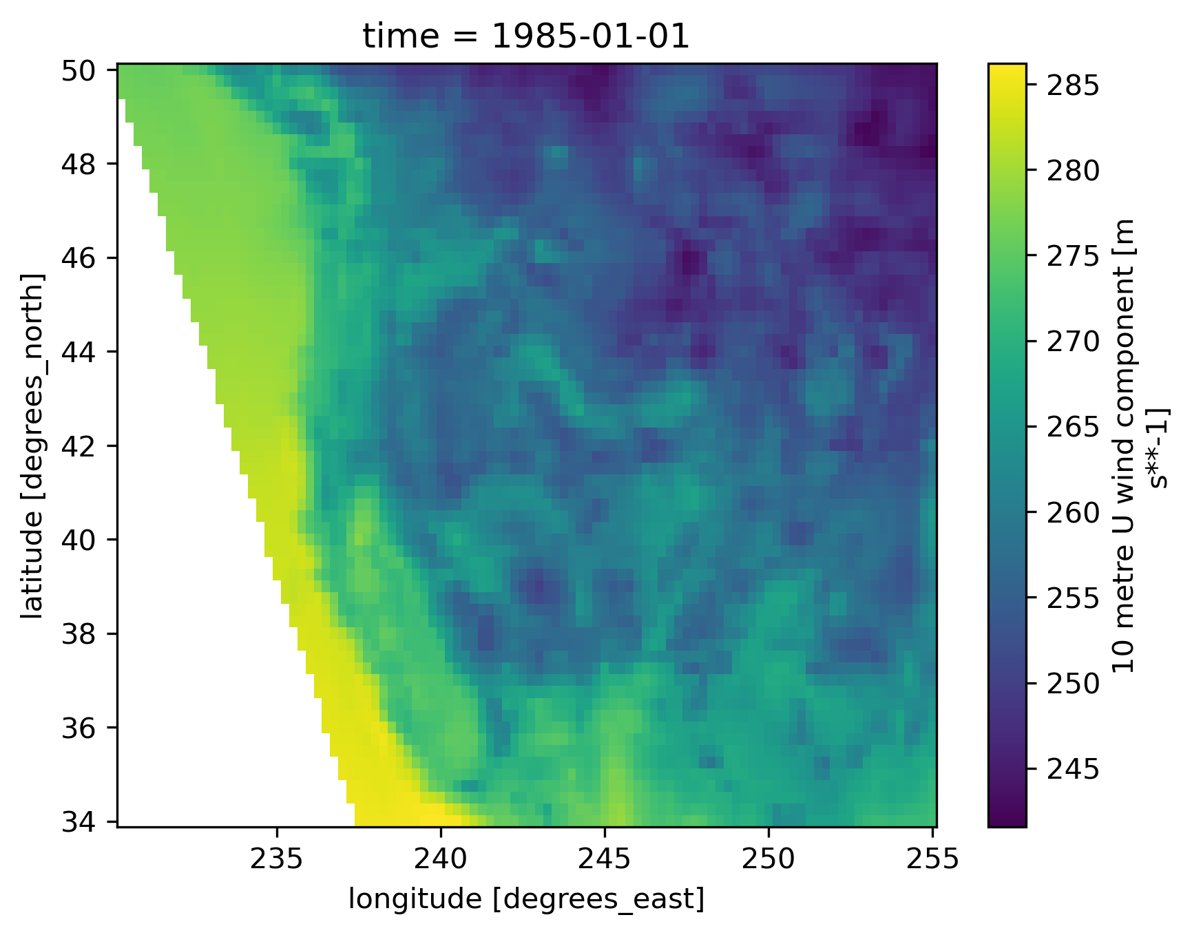
We can see that this is a subset of the oeverall dataset given the number of latitude and longitude values remaining, and their values tend to match up to what we want, but it’s worth making sure things look reasonable before we move on to the rest of the processing pipeline. Here we just show a single map of the data for the first timeset, and can make out most of the major features of the western North America, including some of the coastal oceans which are included before masking things out.
subset['tasmin'].isel(time=0).plot()
<matplotlib.collections.QuadMesh at 0x7fcf10450d60>
So far we have a simple and scalable first step to being able to process this data quickly, since this selection method is lazy and means we can reach this point with almost no actual underlying computation. The next step that is reasonable to ask is: given this as our modeling domain, what does an actual “sample” consist of? Since we are still dealing with a relatively coarse spatial scale we will assume that we can neglect spatial redistribution of snow via wind and other processes. But, because snow accumulation and ablation processes can occur over long time periods we will need to account for time explicitly. That means that we will consider a single sample to be a single grid cell with some time history. We’ll get a bit more into how this is actually represented in the model later, but for now we can summarize that we want to select out a single location from the model for a specified period of time. We will use the xbatcher python package to actually facilitate this.
Given we have the zen3geo package also installed from the setup cells xbatcher and the torchdata.datapipes are already interoperable via the pipe.slice_with_xbatcher method. We simply have to define some dimensions to consider a sample and we are good to go. But, before we do that, it’s worth taking a moment to discuss samples versus batches. A sample is considered an individual example of the mapping that we want the model to learn. Ideally we could process all samples simultaneously to optimize our model, but as in many other areas where machine learning is common, this is computationally intractable for use. As an alternative to “full batch” processing we use the now standart approach of “mini batch” processing where we group together a small fraction of the total samples available to provide to the model and optimization routine at each update step. This is the reason that learning across large datasets is possible, and we implement this in a simple manner by grouping together nearby gridcells - often referred to as “chunks”, “patches”, or most commonly in the geospatial community as “chips”.
This is all handles behind the scenes by xbatcher simply by specifying the batch_dims. The time period that we consider relevant is specified via the input_dims argument. We consider this to be 180 days here as a “naive” choice because we have chosen our gridcells of interest to be locations where snow is common, but not present year-round in the ERA5 data. This is a “hyperparameter” that is ripe for further testing.
input_dims={'time': 180}
batch_dims={'lat': 30, 'lon': 30}
input_overlap={'time': 45}

pipe = RegionalSubsetterPipe(ds, ['WNA'])
pipe = pipe.slice_with_xbatcher(
    input_dims=input_dims,
    batch_dims=batch_dims,
    input_overlap=input_overlap,
    preload_batch=False
)
for batch in pipe:
    b = batch
    break

b
<xarray.Dataset>
Dimensions:        (time: 180, sample: 900)
Coordinates:
  * time           (time) datetime64[ns] 1985-01-01 1985-01-02 ... 1985-06-29
  * sample         (sample) object MultiIndex
  * lat            (sample) float32 50.0 50.0 50.0 50.0 ... 42.75 42.75 42.75
  * lon            (sample) float32 230.2 230.5 230.8 ... 237.0 237.2 237.5
Data variables: (12/21)
    pr             (sample, time) float64 dask.array<chunksize=(900, 180), meta=np.ndarray>
    ps             (sample, time) float32 dask.array<chunksize=(900, 180), meta=np.ndarray>
    psl            (sample, time) float32 dask.array<chunksize=(900, 180), meta=np.ndarray>
    rsds           (sample, time) float64 dask.array<chunksize=(900, 180), meta=np.ndarray>
    tas            (sample, time) float32 dask.array<chunksize=(900, 180), meta=np.ndarray>
    tasmax         (sample, time) float32 dask.array<chunksize=(900, 180), meta=np.ndarray>
    ...             ...
    aspect_sine    (sample) float64 nan nan nan nan ... 0.02424 0.008986 -0.2774
    elevation      (sample) float64 nan nan nan nan ... 734.1 839.2 1.094e+03
    slope          (sample) float64 nan nan nan nan ... 11.36 10.05 8.716 6.84
    mask           (sample) float64 0.0 0.0 0.0 0.0 0.0 ... 1.0 1.0 1.0 1.0 1.0
    cbrt_swe       (sample, time) float32 dask.array<chunksize=(660, 46), meta=np.ndarray>
    cbrt_pr        (sample, time) float64 dask.array<chunksize=(900, 180), meta=np.ndarray>
Attributes:
    institution:  ECMWF
    source:       Reanalysis
title: ERA5 forecastsFrom this you can see that xbatcher has automatically flattened out the latitudes and longitudes into a single sample dimension. But, given that our selection from the regionmask utility is a square bounding box over the full dataset we still have to consider if all of the data in the sample dimension is valid. We will filter this data out with a function that removes any gridcells that do not lie within our predefined mask. This ends up being a simple boolean mask check:
def filter_batch(batch):
    return batch.where(batch['mask']>0, drop=True)
We can then incorporate this into our data processing pipeline simply by calling the .map method on our existing pipeline objects with this function as the argument. We will hold off on demonstrating this until we have completed the last two steps of the pipeline, but feel free to experiment with the final code we provide to see how this works in practice.
The next question is, given a batch of data to be fed into a model, do we need to do any “postprocessing” first? Generally it is necessary to scale data to be approximately normalized for deep-learning based models to train effectively. This is no exception in Earth/environmental science applications where inputs/covariates can often span multiple orders of magnitude. We’ll use the basic standardization technique where we subtract the mean of the data and divide by the standard deviation for each variable. This sits atop an assumption that our data is somewhat normally distributed, which is certainly not true for all variables but we can get around by making some deliberate choices for scale factors. This would be a ripe area for further exploration, and can result in some nice boosts to both model training speed and end model performance at the end of the day, but can get a bit complex for our purposes here so we leave improvements and tweakes as next steps.
def transform_batch(batch):
    scale_means = xr.Dataset()
    scale_means['mask'] = 0.0
    scale_means['swe'] = 0.0
    scale_means['pr'] = 0.00
    scale_means['tasmax'] = 295.0
    scale_means['tasmin'] = 280.0
    scale_means['elevation'] = 630.0
    scale_means['aspect_cosine'] = 0.0

    scale_stds = xr.Dataset()
    scale_stds['mask'] = 1.0
    scale_stds['swe'] = 3.0
    scale_stds['pr'] = 1/100.0
    scale_stds['tasmax'] = 80.0
    scale_stds['tasmin'] = 80.0
    scale_stds['elevation'] = 830.0
    scale_stds['aspect_cosine'] = 1.0
    # Just do a simple standardization
    batch = (batch - scale_means) / scale_stds
    return batch
Nice - we’re almost there! Last thing we have to do is actually split the data out into our inputs/outputs. This point is where we have to actually come face-to-face with the data and finally get it into the format that the ML model expects.
At this point we’ve got a data pipeline that can open the data, slice it up into samples, filter out missing samples, and normalize the data. This is all done as an xarray.DataSet, which will first need to be stacked together so all of the variables are part of a single array, and then we will need to make sure that the dimension order matches what our model will expect. For the moment that step will be a leap of faith, but you will see how things pan out in the next portion of the tutorial. Finally, we just need to convert things to a torch.tensor so that we can actually take advantage of the PyTorch ecosystem. As a final note, we have implemented things so that if the number of samples is less than some threshold we just skip that batch. This is because our mask was irregular and it’s generally not worth running very small samples through our model for training.
def stack_split_convert(
    batch,
    in_vars,
    out_vars,
    in_selectors={},
    out_selectors={},
    min_samples=200
):
    dims = ('sample', 'time', 'variable')
    if len(batch['sample']) > min_samples:
        # Go from a dataset which has multiple variables
        # to a single dataarray, which stacks the variables.
        # Then, transpose them to the desired order for the
        # model in the next step.
        x = (batch[in_vars]
              .to_array()
              .transpose(*dims))
        y = (batch[out_vars]
              .to_array()
              .transpose(*dims))
        # Convert to `torch.tensor`
        # The call `x.values` converts from xarray to numpy
        # Then following that we convert to the tensor
        # Finally we make sure that we are using 32 bit floats
        x = torch.tensor(x.values).float()
        y = torch.tensor(y.values).float()
    else:
        # Just return an empty tensor so we can skip later
        x, y = torch.tensor([]), torch.tensor([])
    return x, y
Now, note that the stack_split_convert function takes many parameters which can be flexibly specified to change how the data comes out. Because pytorch data pipes can only be functions of a single variable, we will need to predefine some of these, and then use a handy tool from the functools module called partial.
To explain the partial function in a concise manner, let’s just go over a simple example. Imagine you have inherited a two argument function aptly named two_arg_fun from a colleague:
def two_arg_fun(a, b):
    return a ** b
And further suppose that you know what b is for your particular case, and it’s a fixed value of 2. Then, it’s not terribly difficult to run this once:
fixed_b = 2
x = np.arange(0, 5, 0.05)
y = two_arg_fun(x, b=fixed_b)
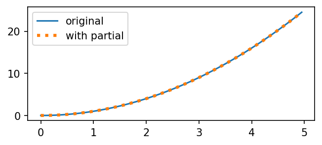
But, where partial comes in is making it easy to define a new function that not only has a name, but can be passed around to other functions. For example, in our very simple case we can reproduce the prevous behavior with:
f, ax = plt.subplots(1, 1, dpi=150, figsize=(5,2))
fixed_fun = partial(two_arg_fun, b=fixed_b)
ax.plot(x, y, label='original')
ax.plot(x, fixed_fun(x), label='with partial', linestyle=':', linewidth=3)
plt.legend()
<matplotlib.legend.Legend at 0x7fcf100b6fa0>
Given that small, practical example let’s get back to our final piece of the data pipeline. We just need to be able to inject variables into the stack_split_convert function. We can define all of them up front, which acts as a nice “configuration” step as we’ll see later. This will define all of the important things for our training workflow like what the inputs and targets/outputs are, sequence lengths, dimensions of our batch sizes, and how much to overlap training samples. With everything configured we can just run it through the partial function with relevant keywords and then we are good to put things together.
in_vars = ['pr',  'tasmax',  'tasmin',  'elevation',  'aspect_cosine']
out_vars = ['swe']
output_sequence_length = 1
output_selector = {'time': slice(-output_sequence_length, None)}
convert = partial(
    stack_split_convert,
    in_vars=in_vars,
    out_vars=out_vars,
    out_selectors=output_selector,
)
Putting it all together#
Wow, it’s been a bit of work to get here, but that’s all of the components for our data processing pipeline. Now we just need to be able to assemble it. We promised that the point of using torchdata.datapipes was to simplify things and now you finally get to see that in action! We have a bit more configuration set up just for example.
regions = ['WNA']
varlist = ['mask'] + in_vars + out_vars
input_sequence_length = 180
input_dims={'time': input_sequence_length}
batch_dims={'lat': 30, 'lon': 30}
input_overlap={'time': 45}
And, we can now actually chain things together and try it out. This is a crucial step in developing your own data pipelines, so make sure to see how each of the above steps is incorporated into the final pipeline of steps below. You can (and should) verify that the pipeline works before you step through to the next notebook, but that’s simple enough.
# Open the data and subset to region
dp = RegionalSubsetterPipe(ds[varlist], regions)
# Generate chips from the region
dp = dp.slice_with_xbatcher(
    input_dims=input_dims,
    batch_dims=batch_dims,
    preload_batch=False
)
# Filter out any missing data
dp = dp.map(filter_batch)
# Transform/normalize the data
dp = dp.map(transform_batch)
# Reshape and convert it to a torch.tensor
dp = dp.map(convert)

x, y = next(iter(dp))
print('Input batch has shape:  ', x.shape)
print('Target batch has shape: ', y.shape)
Input batch has shape:   torch.Size([232, 180, 5])
Target batch has shape:  torch.Size([232, 180, 1])
Automating the data pipeline creation#
Now that we have a full workflow in place it is good practice to wrap things up into a nice function so that it can be used in future workflows/scripts/notebooks. For completeness we show how to wrap all of this up, and also show how this can be used as a library function. This is all implemented in the src.datapipes module which will be imported in our training routines and beyond, so make sure to look at how the implementations are similar.
def make_data_pipeline(
    ds,
    regions,
    input_vars,
    output_vars,
    input_sequence_length,
    output_sequence_length,
    batch_dims,
    input_overlap,
):
    # Preamble: just set some stuff up
    output_selector = {'time': slice(-output_sequence_length, None)}
    input_dims={'time': input_sequence_length}
    varlist = ['mask'] + input_vars + output_vars
    convert = partial(
        stack_split_convert,
        in_vars=input_vars,
        out_vars=output_vars,
        out_selectors=output_selector,
    )
    # Chain together the datapipe
    dp = RegionalSubsetterPipe(ds[varlist], selected_regions=regions)
    dp = dp.slice_with_xbatcher(
        input_dims=input_dims,
        batch_dims=batch_dims,
        input_overlap=input_overlap,
        preload_batch=False
    )
    dp = dp.map(filter_batch)
    dp = dp.map(transform_batch)
    dp = dp.map(convert)
    return dp
As a last step you can see how we can instantiate the entire workflow pipeline and finally iterate over it. This provides the baseline for the model that we’ll train, and is a great achievement to have completed. Frankly, setting up the data processing pipeline can be one of the most onerous and tricky parts of a machine learning pipeline. Make sure that you spend appropriate time here before diving straight into trying to train/fit your model because, as they say, “garbage in = garbage out”.
p = make_data_pipeline(
    ds, ['WNA'], in_vars, out_vars,
    input_sequence_length, output_sequence_length,
    batch_dims, input_overlap
)
x, y = next(iter(p))
print(x.shape, y.shape)
torch.Size([232, 180, 5]) torch.Size([232, 180, 1])